
NPC Editor's Note: This document is under construction and has not been check for accuracy with the original.
ESL-ET59
28 June 1973
Sea-Tac AIR QUALITY - FINAL
R. Adams
B. Hulet
D. Ramras
H. Seidman
| Contents | ||
| Section | Page | |
| 1. | Introduction | 1-1 |
| 1.1 | Carbon Monoxide | 1-3 |
| 1.1.1 | Sources | 1-3 |
| 1.1.2 | Carbon Monoxide Chemsitry | 1-4 |
| 1.1.3 | Effects of Carbon Monoxide | 1-4 |
| 1.2 | Hydrocarbons | 1-5 |
| 1.2.1 | Sources | 1-7 |
| 1.2.2 | Hydrocarbon Chemistry | 1-7 |
| 1.2.3 | Effects of Hydrocarbons | 1-8 |
| 1.3 | Nitrogen Oxides | 1-9 |
| 1.3.1 | Sources | 1-9 |
| 1.3.2 | Chemical Interactions of Nitrogen Oxides in the Atmosphere | 1-10 |
| 1.3.3 | Effects of Nitrogen Oxides | 1-11 |
| 1.4 | Photochemical Oxidants | 1-11 |
| 1.4.1 | Sources | 1-13 |
| 1.4.2 | Effects of Photochemical Oxidants on Vegetation, Materials, and Animals | 1-13 |
| 1.5 | Particulate | 1-15 |
| 1.5.1 | Sources | 1-15 |
| 1.5.2 | Effects of Particulate Matter | 1-16 |
| 1.6 | Ambient Air Quality Standards | 1-17 |
| 1.7 | References | 1-22 |
| 2. | Existing Air Quality | 2-1 |
| 2.1 | Topographical and Climatic Conditions | 2-1 |
| 2.2 | Meteorology | 2-2 |
| 2.2.1 | Mixing Depth and Turbulence Classification Near Sea-Tac | 2-4 |
| 2.3 | Archival Air Quality | 2-8 |
| 2.4 | Meteorological PArameters and Air Pollution Levels At Sea-Tac | 2-10 |
| 2.4.1 | Location of Ambient Air Quality Measurements Near Sea-Tac | 2-10 |
| 2.4.2 | Existing Air Quality - Carbon Monoxide (CO) | 2-11 |
| 2.4.3 | Existing Air Quality - Hydrocarbons | 2-13 |
| 2.4.4 | Existing Air Quality - Nitrogen Dioxide | 2-17 |
(NPC Editor's Note: the page labeled "ii" was missing and thus could not be published. We apologize for any inconvenience this may bring about. We are currently seeking the page)
| Contents --Continued | ||
| Section | Page | |
| 7. | Mitigation Measures to Improve Air Quality at Sea-Tac | 7-1 |
| 7.1 | Aircraft Source Controls | 7-2 |
| 7.2 | Mobile Source Controls | 7-6 |
| 7.3 | Land-Use Alternatives | 7-7 |
| 7.4 | Conclusions | 7-9 |
| 7.5 | References | 7-9 |
(NPC Editor's Note: the page labeled "iv" was missing and thus could not be published. We apologize for any inconvenience this may bring about. We are currently seeking the page)
| Illustrations --Continued | ||
| Figure | Page | |
| 5-2. | Predicted 1973 Worst Case CO Isopleths mg/m3 (1 Hour Maximum) | 5-4 |
| 5-3. | 1973 Hydrocarbon Isopleths 3 - Hour Average 6-9 A.M. Average Conditions µg/m3 | 5-6 |
| 5-4. | 1973 Hydrocarbon Isopleths 3 - Hour Average 6-9 A.M. Worst Case Conditions (HC) µg/m3 | 5-7 |
| 5-5. | 1973 NOx Isopleths Near Sea-Tac Annual Average µg/m3 | 5-8 |
| 5-6. | 1973 Particulate Isopleths Annual Geometric Mean µg/m3 | 5-11 |
| 5-7. | 1973 Worst Case 24 - Hour Particulate µg/m3 | 5-13 |
| 6-1. | Sea-Tac Aircraft Emission Trends 1973-1993 | 6-9 |
| 6-2. | Predicted CO Isopleths (Average Conditions - 8 Hours mg/m3) | 6-15 |
| 6-3. | Predicted CO Isopleths (Worst Case Conditions - 1 Hour µg/m3) | 6-16 |
| 6-4. | Predicted Hydrocarbon Isopleths (3 - Hour Average, 6-9 A.M., Average Conditions, µg/m3) | 6-17 |
| 6-5. | Predicted Hydrocarbon Isopleths (3 - Hour Average, 6-9 A.M., Average Conditions µg/m3) | 6-18 |
| 6-6. | Predicted NOx Isopleths (Annual Average µg/m3) | 6-20 |
| 6-7. | Predicted Particulate Isopleths (Annual Geometric Mean µg/m3) | 6-22 |
| 6-8. | Predicted Particulate Isopleths (Worse Case, 24 - Mean Average µg/m3) | 6-23 |
| 7-1. | Hydrocarbon and Carbon Monoxide Emissions From a Typical Aircraft Engine (JT3D) | 7-4 |
| TABLES | ||
| Table | Page | |
| 1-1 | Nation-Wide Emission Estimates, 1970 | 1-2 |
| 1-2 | Representative NO2 Effects | 1-12 |
| 1-3 | Effects Associated with Exodant Concentrations in Photochemical Smog | 1-14 |
| 1-4 | Effects Associated with PArticulate Levels | 1-17 |
| 1-5 | National Primary and SEcondary Ambient Air Quality Standards | 1-19 |
| 2-1 | Average Mixing Depths and Wind Speeds at Sea-Tac Airport | 2-4 |
| 2-2 | Relation of Pasquill Turbulence Types to Weather Conditions | 2-6 |
| 2-3 | Frequency Distribution of Pasquill Turbulence Types at Sea-Tac International Airport, January 1 - December 31, 1969 | 2-6 |
| 2-4 | Summary of Puget Sound Air Pollution Control Agency Data Near Sea-Tac | 2-9 |
| 2-5 | Elemental Analysis of Particulate at Sea-Tac Compared to Rural Area in California | 2-26 |
| 2-6 | Average Daytime Carbon Monoxide Levels Around Sea-Tac Terminal | 2-28 |
| 2-7 | Average Daytime CO Levels Sea-Tac Environs | 2-29 |
| 3-1 | Modal Emission Factors - EPA (lbs/hr) and Sea-Tac Modal Emissions (lbs) | 3-3 |
| 3-2 | Average Time Assigned to Aircraft Operating Modes at Various Airports | 3-4 |
| 3-3 | Air Carrier Operations Sea-Tac 1972 | 3-6 |
| TABLES --Continued | ||
| Table | Page | |
| 3-4 | Total Engine LTOs Sea-Tac Airport 1972 | 3-7 |
| 3-5 | 1973 Aircraft Emissions at Sea-Tac | 3-8 |
| 3-6 | Aircraft Emissions at Sea-Tac and Other Airports | 3-10 |
| 3-7 | 1973 Vehicular Emissions at Sea-Tac | 3-13 |
| 3-8 | Annual Emissions at Sea-Tac Due to Aircraft and Motor Vehicles (Tons/Year) | 3-13 |
| 3-9 | Emission Factors for Fuel Oil and Natural Gas Combustion | 3-14 |
| 3-10 | Total Emission for Fuel Oil and Natural Gas Combustion | 3-15 |
| 6-1 | Proposed Aircraft Emissions Standards | 6-2 |
| 6-2 | Sea-Tac Air Traffic Forecasts | 6-4 |
| 6-3 | Sea-Tac Aircraft Mix | 6-4 |
| 6-4 | Sea-Tac Engine LTOs | 6-5 |
| 6-5 | Modal Emission Factors - EPA (lbs/hr) and Sea-Tac Modal Emissions (lbs) | 6-6 |
| 6-6 | Predicted Sea-Tac Emissions (Tons/Yr) | 6-7 |
| 6-7 | Sea-Tac Predicted Aircraft Emissions (Without Emission Controls) | 6-9 |
| 6-8 | Computation of Sea-Tac Automobile Emissions Associated with Passengers and Employees | 6-10 |
| 6-9 | Ground Service Vehicle Emissions | 6-12 |
| 6-10 | Predicted Sea-Tac Emissions 1973-1993 | 6-13 |
1. Introduction
Numerous definitions of air pollution have been devised depending upon a particular author's perspective. In general, pollutants are considered to be those substances present in sufficient concentrations to produce a measurable effect on man, animals, vegetation, or materials. Air pollutants may, therefore, include almost any material or artificial composition of matter capable of being airborne. They may be present as solids, liquids or gases, or mixtures; and some classification or categorization is required.
Two general groups of air pollutants are recognized: (a) those emitted directly from identifiable sources and (b) those produced in the air by interactions among two primary pollutants, or by reactions between primary pollutants and normal atmospheric constituents. At the present time, the primary air pollutants are identified as carbon monoxide (CO), sulfur dioxide (SO2), nitrogen dioxide (NO2), particulate matter (PM), and hydrocarbons (THC = total hydrocarbons: HC = hydrocarbons less methane). Secondary air pollutants are grouped together as photochemical oxidants (Ox) and include ozone, alkyl nitrates, peroxyacyl nitrates (PAN), alcohol, ethers, acids, and peroxyacids. Although this classification is useful, it should be recognized that certain sources may emit secondary pollutants directly; and depending on the measurement techniques being used, some secondary pollutants may be counted twice or not at all.
Several attempts have been made to estimate the major source categories contributing the primary air pollutants. A recent attempt (1970) is shown in Table 1-1. From the table it can be seen that on a mesoscale basis, aircraft contribute only 0.3 to 2 percent of the total primary emissions. However, on a microscale basis at or near am ai1-port, these small amounts may be sufficient to generate hazardous levels of primary pollutants and contribute to the formation of secondary pollutants.
Table 1-1. --Nation-Wide Emission Estimates, 1970
Pollutant Emissions Source Category |
SOx
34 x 105 Tons/Year % of Total |
Particulate
26 x 106 Tons/Year % of Total |
CO
149 x 106 Tons/Year % of Total |
HC
35 x 106 Tons/Year % of Total |
NO2
23 x 105 Tons/Year % of Total |
| Transportation | 3.0 | 2.7 | 74.5 | 55.9 | 51.3 |
| -Motor Vehicles | 0.9 | 1.5 | 64.8 | 47.9 | 39.9 |
| --Gasoline | 0.6 | 1.1 | 64.3 | 47.6 | 34.2 |
| --Diesel | 0.3 | 0.4 | 0.5 | 0.3 | 5.7 |
| -Aircraft | 0.3 | 0.4 | 2.0 | 1.1 | 1.8 |
| -Railroads | 0.3 | - | 0.1 | 0.3 | 0.4 |
| -Vessels | 0.9 | 0.4 | 1.2 | 0.9 | 0.9 |
| -Nonnignway use of motor fuels | 0.6 | 0.4 | 6.4 | 5.7 | 8.3 |
| Fuel combustion in stationary sources | 78.1 | 26.1 | 0.6 | 1.7 | 43.8 |
| -Coal | 65.4 | 21.5 | 0.3 | 0.6 | 17.1 |
| -Fuel oil | 12.4 | 1.5 | 0.1 | 0.3 | 5.7 |
| -Natural gas | - | 0.8 | 0.1 | 0.8 | 20.6 |
| -Wood | 0.3 | 2.3 | 0.1 | - | 0.4 |
| Industrial process losses | 17.7 | 51.0 | 7.7 | 15.8 | 0.9 |
| Solid waste disposal | 0.3 | 5.3 | 4.9 | 5.7 | 1.8 |
| Agricultural burning | 0.3 | 9.2 | 9.3 | 8.0 | 1.3 |
| Miscellaneous | 0.6 | 5.7 | 3.0 | 12.9 | 0.9 |
| -Forest fires | - | 5.3 | 2.7 | 0.9 | 0.9 |
| -Structural fires | - | - | 0.1 | 0.3 | - |
| -Coal refuse burning | 0.6 | 0.4 | 0.2 | 0.3 | - |
| -Gasoline & solvent evaporation | - | - | - | - | - |
1.-- Continued.
In order to understand the intent and importance of Federal air quality standards, it is necessary to be knowledgeable about the primary and secondary pollutants. The next few sections briefly discuss each of the air pollutants associated with aircraft operations with respect to their source, chemistry, and effects. A final section relates the Federal standards to the current understanding of air pollution causes and effects.
Most carbon monoxide is produced when there is incomplete combustion of
hydrocarbon fuels. The normal combustion products are carbon dioxide and
water vapor, but a shortage of oxygen or the characteristics of the
combustion processes will generate CO. Total emissions of CO exceed those
of all other pollutants combined.
At the present time, natural sources of CO are considered insignificant,
and most atmospheric CO is produced by the incomplete combustion of
gasoline in motor vehicles (65 percent). Other transportation sources
account for 10 percent, agricultural burning 9 percent, industrial
process-losses 8 percent, and miscellaneous another 8 percent. Only 2
percent of the total is associated with aircraft.
Carbon monoxide is a colorless, odorless, tasteless is slightly lighter
than air. Although it does not support combustion, it is quite flammable.
Reactions between CO and atmospheric components do not occur because of
high activation energies required. Thus, the conversion of CO to CO2
(carbon dioxide) by ozone has an activation energy ten times that of the
comparable reaction between nitric oxide (NO) and ozone. other reactions
such as oxidation by nitrogen dioxide NO2 also have high
activation energies. At the present time, several removal mechanisms are
postulated to account for the relatively constant background CO levels in
the absence of known removal processes.
It has not been demonstrated that Co produces adverse reactions in higher
types of plant life at concentrations which reduce loss of consciousness
or death in animals. The possible effects of high CO levels within the
soil has not been thoroughly investigated, but significant impact on
vegetation and micro- organisms at ambient levels is unlikely.
The toxicological properties of CO are associated with its absorption in the lungs and subsequent reaction with hemo proteins. Most significantly, the iron containing hemoglobin molecule forms a stable complex with CO because of theavailable electron pair on CO. The strength of the affinity is great enough to displace the oxygen molecule from oxyhemoglobin, thereby forming carboxyhemoglobin (COHb). Hypoxia or diminished availability of oxygen to the cells of the body results, Figure 1-1 summarizes the known effects of short term exposures to CO levels in terms of the blood C0Hb levels observed, The ambient concentrations of CO necessary to result in these blood C0Hb levels are a function of ventilation rate and length of exposure. Generally, it will take 8 hours or more to reach equilibrium between ambient CO levels and blood COHb levels. Given sufficient exposure time, and assuming a background COHb level of 0.5percent, the equilibrium percent COHb can be estimated for ambient levels of CO (less than 115 mg/m3 or 100 ppm) from: COHb percent = 0.16 CO ppm + 0.5. Thus, in Figure 1-1 a 50 ppm CO exposure for more than 8 hours is roughly equivalent to 8.5 -percent COHb. This figure can be compared to moderate smokers whose median COHb level may run 6 percent.
Certain organic compounds contain only two elements, hydrogen and carbon,
and hence are known as hydrocarbons (HC). On the basis of structure,
hydrocarbons are divided into two main Classes: aliphatic and aromatic.
Aliphatichydrocarbons are further divided into families: alkanes
(saturated), alkenes, and alkynes. Hydrocarbon
oxidation products such as aldehydes, acetones, peroxides, and others
play an important role in the
Figure 1-1. Effects of CO on Human Health. From: Philip C. Wolf, Carbon Monoxide, Measurement and Monitoring in Urban Air
1.2 --Continued.
photochemical system of the atmosphere. Unlike carbon monoxide and nitrogen oxides, hydrocarbon criteria are not based on direct effects, but on their role as precursors of other damaging compounds formed in the photochemical system.
Natural sources, particularly biological processes, account for a large
proportion of hydrocarbon emissions. Non- urban air typically contains 0.7
to 1.0 mg/m3 methane (1.0 to 1.5 ppm) and less than 0,1 ppm
each of other hydrocarbons.
Technological emissions of hydrocarbons. are estimated at 34.9 x 10⁶ tons/year. Transportation represents the largest source category and accounts for 56 percent of this estimate (1970) only. 1 percent of the total is believed to be associated with aircraft, other significant sources are: industrial process losses (16 percent), gasoline and solvent evaporation (11.4 percent and non-highway use of motor fuels (6 percent). HC emissions, therefore, originate primarily from inefficient combustion of gasoline and from their use as process raw materials.
Hydrocarbons in the urban atmosphere are comprised primarily of alkanes
(with or without methane) followed by the aromatics, alkenes, and alkynes.
For example, several hundred samples from one urban location had the
following composition (mq/m3 as carbon): methane 2.10, other
alkanes 0.90, aromatics 0.37, and alkene (ethylene) 0.08. It is somewhat
heuristic to distinguish hydrocarbons at this time, even though their
relative importance in the photochemical system may be significant,
because existing standards specify allowable levels for focal hydrocarbons
less methane. In the future, separate standards may exist which could
reorder the significance of hydrocarbon sources.
The complexity of the photochemical system has prevented a complete understanding of the relationship betweenhydrocarbon levels and ambient air quality. As a result, an empirical approach has developed of comparing the 6:00 to 9:00 AM average hydrocarbon values with hourly maximum oxidant values obtained later in the day. Large amounts of data collected from numerous cities is the basis for comparing early morning HC levels to peak oxidant levels. These observations have revealed that if the 6:00 to 9:00 AM non methane hydrocarbon level is below 200 µg/m3 (0.3 ppm), maximum oxidant levels will stay below 200 µg/m3 (0 .10 ppm).
At ambient concentrations, ethylene is the only known Hydrocarbon to have
adverse effects on certain types of vegetation. Ethylene may cause
abnormal leaf growth and abscission of leaves, flower buds, and flowers,
as well as growth inhibition.
At the present time, there are no known adverse health effects associated with high concentrations of hydrocarbons in the ambient air. However, their involvement in the formation of oxidants and other hazardous derivatives requires that they be considered pollutants.
Of the eight nitrogen oxides known to exist, two -Nitric oxide and
nitrogen dioxide- are emitted to the atmosphere in significant quantities.
Ambient air contains nitrogen (78 percent by volume) and oxygen (20
percent by volume). As a result, any atmospheric combustion process
produces nitrogen oxides. The amount formed depends on the combustion
temperature, the concentration of both reactants and products, and other
combustion conditions.
Combustion temperatures in excess of l100·C produce NO and NO2 (usually less than 0.5 percent). NO is rapidly converted to NO2 by atmospheric oxygen (O2) when NO concentrations exceed 1 ppm and more slowly via a photochemical cycle at lower concentrations.
Fuel combustion from transportation sources and from stationary sources accounts for 51 percent and 44 percent respectively of the nationwide emissions of nitrogen oxides. Of the transportation sources, motor vehicles contribute 40 percent (78 percent of 51 percent) of the emissions and aircraft 1.8 percent. Residential fuel consumption accounts for only 25 percent of the emissions, while power generating stations and industrial users account for die remaining 41 percent.
Ultraviolet light from the sun reacts with nitrogen dioxide causing it to
dissociate into nitric oxide and atomic oxygen. Ozone is formed when
atomic oxygen reacts with atmospheric oxygen, The remaining chemistry is
complex and not yet completely understood. However, the interaction of
certain hydrocarbons (HC) with the by-products of the photo- dissociation
of NO2 is believed to result in the formation of reactive free
radicals. These free radicals and others formed via different mechanisms
are highly reactive and may combine with oxygen (O2), NO2
or NO to form peroxy radicals, peroxyacyl nitrates (PAN, an eye irritant),
and additional NO2. As a result, NO is converted to NO2
which is itself destroyed via photodissociation and reaction with other
pollutants to produce ozone and organic nitrates.
Significant effects of NOx (NO2 + NO) have been
observed and studied on textile dyes, natural and synthetic fibers, and
metals, color loss has been observed in gas dryers where NOx
concentrations range from 1.1 to 3.7 µg/m3, cotton and
nylon textile fiber deterioration is known; but specific thresholds have
not been determined.
High concentrations of NO2 (47 mg/m3) for any extended period of time produce accute necrotic leaf injury. The effects of exposure to low levels of iio2 for extended periods are less evident. studies indicate that levels below 470 µg/m3 supplied for a period of 8 months will cause increased leaf damage and reduced yield in navel oranges.
Low levels of NO2 (0.04 ppm) are associated with the formation of photochemical oxidant above the Federal Standard. Between 0.067 and 0,109 ppm, NO2 causes increased respiratory disease. These and other known effects aresummarized in Table 1-2.
Photochemical oxidants result from a complex series of atmospheric
chemical reactions initiated by sunlight. Aldehydes, acetones, nitrogen
dioxide, and other compounds absorb ultraviolet energy from the sunlight
and dissociate into reactive free radicals. The free radicals initiate
reaction chains that lead to the formation of new compounds; including
onone, peroxyacyl nitrates, alcohols, ethers acids and peroxyacids.
Table 1-2. Representative NO2 Effects
(NPC Editor Note: Our copy of this document was partially illegible: An updated version is being sought. We apologize for any aggravation this may cause)
| Effect
Lowest Level Associated with Reference Oxidant Production of ??? µg/m3 |
NO2 Concentration ppm
0.04 |
NO2 Concentration -g/m3
80 |
Duration
3 Hr. (6 to 9 A.M.) |
Comment | Reference
1 |
| Increased incidence of acute respiratory disease in families | 0.067 to 0.109 | 117 to 205 | 2 to 3 Yr. | Chattanooga study - 6 months mean concentration range | 2 |
| Increased incidence of acute bronchitis in infants and school children | 0.063 to 0.083 | 118 to 156 | 2 to 3 Yr. | Chattanooga study - 6 months mean concentration range | 3 |
| Human olfactory threshold | 0.12 | 225 | - | Immediate perception | 4 |
| Rabbits - structural changes in | 0.25 | 470 | 4 hr/day
for 6 days |
Still apparent 7 days after final exposure | 5 |
| Navel orange - Leaf abscission
decreased yield |
0.25 | 470 | 8 months continuously | 6 | |
| Rats - morphological changes in lung mast cells characterized by degranulation | 0.5 | 940 | 4 hr | Possible precedes onset of acute inflammatory reaction | 7 |
| 1.0 | 1880 | 1 hr | |||
| Mice - pneumonitis: alveolar distention | 0.5 | 940 | 6 to 24 hr/day for 3 to 12 months | Possibly emphysematous condition | 8 |
| Mice - increased susceptibility to respiratory infection | 0.5 | 940 | 6 to 24 hr/day up to 12 months | Based on mortality following challenge with K. pneumoniae | 9 |
| Navel orange - Leaf abscission, onlorosis | 0.5 | 940 | 35 days continuously | - | 6 |
| Rats - tachyphea, terminal bronchiolar hypertrophy | 0.8 | 1504 | Lifetime continuously | - | 10 |
Ozone is formed naturally at very high altitudes by solar radiation and by electrical discharge in the atmosphere. These processes are not believed to contribute significantly to urban concentrations. However, ozone levels between 20 and 100 µg/m3 (0.01 to 0.05 gem) have been observed in non-urban areas.
It is important to realize t-hat oxidants (Ox) are secondary pollutants derived from the reactionary of primary pollutants (HC, NOx, SOx ). As such, sources cannot be singled out as was done for hydrocarbons and nitrogen oxides. However, if transportation accounts for 56 percent of the hydrocarbons and 51 percent of the nitrogen oxides, and these pollutants are the precursors of photochemical oxidants; then it is reasonable to associate at least 50 percent of the oxidants with transportation sources.
Many Types times of plants are sensitive to photochemical air pollution.
Ozone injury to leaves in sensitive species will occur after exposure to
60 µg/m3 (0.03 ppm) for 8 hours. Similar injury has been
observed after a 4-hour exposure to 100 µq/m3 (0.05 ppm)
total oxidant. When plants were exposed to ozone for 1 to 4 hours, damage
occurred in highly sensitive plants at levels of 100 to 500 µg/m3
(0.05 - 0.25 ppm), in moderately sensitive plants at 200 to 800 ug/m3
(0.10 - 0.40 ppm), and in resistant giants at 400 µg/m3
and up.
Many materials, particularly organic polymers, are sensitive to even small concentrations of ozone. Economically, rubber is probably the most important material sensitive to ozone attack. As a result, expensive anti-ozonant additives, capable of protecting elastomers, have been developed, at least on a temporary basis. other types of fibers and dyes are also susceptible to ozone attack.
The major physiological effects of ozone are on the respiratory system. Exposure to high levels of ozone (5,900 uq/m3) for several hours produces hemorrhage and edema in the lungs. Lower concentrations of 390 µg/m3 (0.2 ppm) for 3 hours per day, 6 days a week, over 12 week period have not produced any apparent effects in humans. Exposure to 590 µg/m3 (0.3 cam) for 8 hours appears to be the threshold for nasal and throat irritation. Even lower levels of oxidant will produce eve Irritation (200 µg/m3 or 0.1 ppm). The major effects of oxidants are summarized in Table 1-3.
Table 1-3. Effects Associated with oxidant Concentrations in Photochemical Smog
| Effect | Exposure
ppm |
Exposure
-g/m3 |
Duration | Comment |
| Vegetation damage | 0.05 | 4 hours | Leaf injury to sensitive species | |
| Eye irritation | Exceeding
0.1 |
Exceeding
200 |
Peak values | Result of panel response Such a peak value would be expected to be associated with a maximum hourly average concentration of 50 to 100 µg/m3 (0.025 to 0.05 ppm) |
| Aggravation of respiratory diseases - asthma | 0.13* | 250 | Maximum daily value | Patients exposed to ambient air. Value refers to oxidant levels at which number of attacks increased |
| Impaired performance of student athletes | 0.03
to 0.08 |
60 to 590 | 1 hour | Such a peak value would be expected to be associated with a maximum hourly average concentration of 100 to 110 µg/m3 (0.05 to 0.06 ppm) |
| *F.S. = 160 -g/m3 0.08 ppm | Exposure for 1 hour immediately prior to race |
Particulate material in the atmosphere is composed of many different
substances. Depending on the location and the
of activity in the area; fluorides, beryllium, lead, asbestos,
organic material, dust, pollen, and even insect parts mail be present in
particulate matter, some of these are known to be toxic at high levels
while others may have toxic effects that have not yet been studied.
Moreover, laboratory studies suggest a synergistic effect between
particulates and gaseous pollutants.
Particulate air pollution refers to any matter of a diameter greater than one micron (1 millionth of a meter) but smaller than 500 microns suspended in the air. Particles of this size will stay suspended for a few seconds to several months.
Extremely small particles of less than 1 µ in diameter enter the
atmosphere through condensation, combustion, and photo-chemical processes.
Particles between 1 µ and 10 µ in diameter usually include local
soil, process dusts, combustion products from local industries, and even
sea salt. Large particles greater than 10µ result from mechanical
processes such as wind erosion, grinding and spraying, and the pulverizing
of materials by vehicles and pedestrians.
Most adverse effects of particulate air pollution on health are
associated with injury to the surfaces of the respiratory system. The
mechanisms governing the deposition, clearance, and retention of inhaled
particles are complex and not completely understood. Injuries mail be
permanent or temporary and the transport of particulate to other portions
of the body may produce secondary effects,
Available epidemiological studies have defined air pollution in terms of particulate and sulfur compounds. Thus, the levels of particulate and sulfur gases define an index of pollution and not a physiochemical entity.
Most of the epidemiological studies on particulate have concerned air pollution episodes in London and New York. British techniques are not entirely comparable with American measurements, but one study suggests that the British method gives lower results. Particulate air pollution study conclusions are summarized in Table 1-4.
High particulate levels are associated with increased deaths and illness. At lower levels children experience a greater incidence of respiratory diseases and the death rate for persons over 50 appears elevated. Levels of 100-200 µg/m3 cansignificantly reduce visibility and sunlight received at the earth's surface, and increase the corrosion of steel. Particulates soil and damage buildings, statuary, and other surfaces. Plant damage may result when particulate plugs leaf stomates preventing the exchange of gases necessary for growth and development.
Table 1-4. Effects Associated with Particulate Levels
| Particulate Level | Sulfur Dioxide Level | ExceEffects | Comment |
| >750 µg/m3
24 hour average |
>715 µg/m3 | Excess deaths and increased illness | British Study |
| >300 µg/m3
24 hour average |
>630 µg/m3 | Acute worsening of chronic bronchitis | British |
| >200 -g/m3
24 hour average |
>250 µg/m3 | Increased absence of industrial workers due to illness | British |
| >100 µg/m3
annual mean |
>120 -mg/m3
annual mean |
Children experience increased incidence of respiratory diseases | British |
| >80 -g/m3
annual mean |
>30 mg/cm3 | Increased death rates for persons over 50 | American Smoking habits unknown |
| 100-150 -g/m3 | - | Sunlight reduction 5-70% depending on season and latitude | Large smoke turbidity |
| >150 µg/m3 | - | Visibility less than 5 miles | Particulate 0.2µ to 3.0µ R.M. < 70% |
| 60-180 -g/m3 | Present | Corrosion of steel and zinc panels accelerated | Sulfur dioxide and moisture required |
| 70 µg/m3
annual mean |
Present | Approximate thresholds for public concern | Other pollutants present |
Under the authority of the Clean Air Act (42 U.S.C. 1857-18571), as
amended by PL 91-604 the Administrator of the Environmental Protection
Agency (EPA) was required to promulgate national primary and secondary
ambient air quality standards.
National primary ambient air quality standards define levels of air Quality which the administrator judges are necessary, with an adequate margin of safety, to protect the public health. National secondary ambient air Quality levels are those which the administrator Feels are necessary to protect the public welfare from any known or anticipated adverse effects of a pollutant.
The objective of ambient air quality standards is to provide a basis for preventing or abating the effects of air pollution, including effects on health, esthetics, and economy. Since their objective is to improve air quality, the standards are not to be construed to allow significant degradation of existing air quality in any portion of any state which new has air quality superior to that stipulated in tie standards (40 CYR 50)
Normally, the standards are expressed in the metric systems mass of contaminant present in one cubic meter of air at reference conditions (25·C and pressure 760 millimeters of mercury). Alternatively, the concentration is reported as volume of pollutant per million volumes of air or pits per million (ppm).
Based on scientific information similar to that presented in this section, the administrator of the EPA has promulgated standards for air pollutants. Standards for the major air pollutants associated with aircraft operations are presented in Table 1-5.
Table 1-5. National Primary and Secondary Ambient Air Quality Standards
| Pollutant | Averaging Time | Primary | Secondary |
| Carbon Monoxide
CO |
8 hours | 10 mg/m3 (9 ppm)
< Once/year |
Same |
| 1 hour | 40 mg/m3 (35 ppm)
< Once/year |
Same | |
| Nitrogen Dioxide
NO2 |
Annual Average | 100 µg/m3
(0.05 ppm) |
Same |
| Hydrocarbon-less Methane
HC |
3 hours
6-9 A.M. |
160 µg/m3
(0.24 ppm) |
Same |
| Photochemical Oxidants
OX Corrected for NO2 - SOX |
1 hour | 160 µg/m3
(0.08 ppm) < Once/year |
Same |
| Particulate Matter
PM |
Annual Geometric Mean | 75 µg/m3 | 60 µg/m3 |
| 24 hours | 260 µg/m3
< Once/year |
150 µg/m3
< Once/year |
|
| Sulfur Dioxide | Annual Average | 80 µg/m3
(0.03 ppm) |
60 µg/m3
(0.02 ppm) |
| 24 hours | 365 µg/m3
(0.14 ppm) |
260 µg/m3
(0.10 ppm) |
1.6 --Continued.
The relationship between the known effects of these pollutants and the standards can be summarized as follows: An 8-hour exposure to 10 µg/m3 (9 ppm) of CO will produce blood levels of C0Hb of approximately 2 percent. This is the threshold for demonstratable effects. Similarly, short term exposures (1 hour) to CO levels greater than 40 µg/m3 (35 ppm) can be expected to produce COHb blood levels approaching 2 percent. Oxidant effects including eye irritation, respiratory problems, and impaired performance are known to occur when levels approach or exceed 200 µg/m3 (0.08 ppm). Nitrogen dioxide effects are known only for long-term exposures to relatively high concentrations. Thus, this standard is specified over a period of 1 year at 100 µg/m3 10.05 ppm). Particulate levels above 80 µg/m3 with sulfation levels of about 30 µg/cm2 are believed to cause increased death rates in persons over 50 years of age.
Ambient hydrocarbon levels are not associated with adverse health effects. The HC standard is based on a large set of field observations which tend to establish maximum Oxidant levels associated with early morning hydrocarbon levels (Figure 1-2). Nitrogen oxides are also involved in oxidant formation as shown by oxidant isopleths in Figure 1-3. These Observations demonstrate that if the HC levels remain below 160 µg/m3 (0.24 ppm) or if the NOx levels remain below 0.025 ppm, the oxidant level will always be below 200 µg/m3 (0.1 ppm). At the present time, the HC standard is used as a guide in achieving oxidant standards.

1.6 --Continued.
Finally, it should be mentioned that the administrator of the EPA has determined that an earlier proposal to establish a precise level of airborne lead (2 µq/m3) as a standard is not acceptable. Instead, to control ambient lead levels, the administrator has proposed a phased reduction of leaded Fuels by 1978 and automobiles that use lead free gasoline after 1975.
1.7 --Preferences.
The dispersion of air pollutants from any source in the atmosphere is
governed primarily by the dynamic and thermal structure of atmospheric
layer adjacent to the ground. It is well known that the major air
pollution episodes have occurred during periods of calm anticyclonic
conditions, when surface wind speeds are less than 3.1 m/sec (7 mph). To
understand and define existing air quality, it is necessary to take into
account the effects of local topography, wind speeds, and vertical
atmospheric temperature structure. Interactions between these weather
systems, of all scales, over a period of time, produce fluctuations in
wind speed and direction (turbulence) continuously. In this section, data
is presented on meteorological parameters and air quality measurements
near Sea-Tac.
2.1 --Topographical and Climatic Conditions. The geographic features important to air quality in the Puget Sound area are the Olympic Mountains to the west and the Cascade Mountain Range to the east. In both mountain ranges there are mountains over 8,000 feet in elevation. Part of the Puget Sound water mass lies to the west of Sea-Tac, while Lake Washington is to the northeast.
Prevailing winds are either from the north or from the south since the
parallel mountain ranges are oriented north- south. Depending on the
mesoscale pressure gradient, local variations in terrain may influence
circulation patterns. This type of effect can be seen clearly in the wind
roses constructed by the Puget Sound Air Pollution Control Agency (PSAPCA)
from measurements taken at Boeing Field and at Seattle-Tacoma Inter-
national Airport (Figure 2-1). These two airports are only six miles
apart, but they are situated in somewhat different topography. The overall
north-south features are common to both, though there are distinctive
differences.
Seasonal wind patterns are pronounced due to the presence of a semi-permanent low pressure area off the coast during the winter which results in prevailing southerly winds. During the summer, prevailing winds bring Pacific air through the Straits of Juan de Fuca over the northern part of Puget Sound, and from the Grays Harbor area south of the Olympic Mountains to the southern part of Puget Sound. Frequently, this results in northerly winds in the upper portions of King County and southwesterly flow over the southern Puget Sound area.
Diurnal variations in wind direction are most pronounced during the summer season. Daytime winds at Sea-Tac typically are northerly while the nighttime winds are predominately southerly.

Figure 2-1. Annual Surface Wind Roses at Two Seattle-Tacoma Area
Airports for Claendar year 1969.
Another parameter useful in the study of air pollution is the depth of
the convective layer or the mixing depth. Its magnitude for a particular
time of day is usually determined from the latest available chart of
height or pressure vs. temperature.
Table 2-1 gives the average mixing depths and mean wind speeds through the mixing layer by season and time of day at the Sea-Tac Airport.
Table 2-1. Average Mixing Depths and Wind Speeds at Sea-Tac Airport*
| A. Average Mixing Depth (Meters) | |||||
| Winter | Spring | Summer | Fall | Annual | |
| Morning | 626 | 681 | 532 | 476 | 578 |
| Afternoon | 585 | 1490 | 1398 | 898 | 1092 |
| B. Average Mixing Layer Wind Speeds (Meters/Sec) | |||||
| Winter | Spring | Summer | Fall | Annual | |
| Morning | 5.1 | 4.6 | 4.0 | 4.3 | 4.5 |
| Afternoon | 4.7 | 5.7 | 4.8 | 4.6 | 4.9 |
*"Mixing Heights, Wind Speeds and Potential for Urban Air Pollution Through the Contiguous United States," George C. Holzworth (Office of Air Programs Publication No. AP-101, EPA).
2.2.1 --Continued.
The appropriate mixing depth from the table is an input parameter to the ESL air quality model discussed in Section 4 of this report.
Atmospheric turbulence can be based on direct measurements of the three-dimensional fluctuations or eddying motions of the air. Direct measurements are expensive and difficult to make, and classifications based on observable parameters have been developed. Six stability categories were proposed by Pasquill to describe the diffusive potential of the lower atmosphere. The categories are specified in terms of wind speed, insolation (i.e., solar radiation), and amount of cloudiness. Tables 2-2 and 2-3 summarize the parameters that characterize each classification and the frequency of occurrence at Sea-Tac. The slightly stable and neutral conditions generally are associated with nighttime conditions. Even so, at Sea-Tac the neutral D condition occurs most frequently during both daytime and nighttime. In terms of air quality, D conditions will generally be associated with air pollutant levels twice those for B conditions if the wind speed is the same. This effect will be somewhat offset by the typically higher wind speeds associated with D conditions.
In addition to the 1969 Sea-Tac archival data we also obtained PSAPCA data from the McMicken Heights monitoring site. The site was located about I mile due east of Sea-Tac airport. All 1973 data taken at this site is summarized in Figure 2-2, top. Meteorological data taken during ESL's sampling periods of June, September, and February is shown in Figure 2-2, bottom. The similarity of the two wind roses in
Table 2-2. Relation of Pasquill Turbulence Types to Weather Conditions
| A - Extremely Unstable conditions
B - Moderately unstable conditions C - Slightly unstable conditions |
D - Neutral conditions*
E - Slightly stable conditions F - Moderately stable conditions |
||||
| Surface wind speed, m/sec (mph) | Daytime Insolation | Nighttime Conditions | |||
| Thin Overcase
or >4/8 Cloudiness** |
<3/8 Cloudiness | ||||
| Strong | Moderate | Slight | |||
| <2 (4.5) | A | A - B | B | - | - |
| 2 (4.5) | A - B | B | C | E | F |
| 4 (9) | B | B - C | C | D | E |
| 6 (13.5) | C | C - D | D | D | D |
| >6 (13.5) | C | D | D | D | D |
*Applicable to heavy overcast, day or night
**Th degree of cloudiness is defined as that fraction of the sky above the local apparent horizon which is covered by clouds
Table 2-3. Frequency Distribution of Pasquill Turbulence Typed at Sea-Tac International Airport, January 1 - December 31, 1969
| Wind Speed (mph) | |||||||
| 0-3 | 4-7 | 8-12 | 13-18 | 19-24 | >24 | Total | |
| A | - | 0.0017 | - | - | - | - | 0.0017 |
| B | 0.0147 | 0.0195 | 0.0137 | - | - | - | 0.0479 |
| C | 0.0036 | 0.0295 | 0.0521 | 0.0087 | - | - | 0.0987 |
| D | 0.0442 | 0.1525 | 0.2560 | .01480 | 0.0175 | 0.0031 | 0.6213 |
| E | 0.0483 | 0.1251 | 0.0569 | - | - | - | 0.2303 |
| - | - | - | - | - | - | - | |
| 0.1108 | 0.3266 | 0.3787 | 0.1567 | ||||

Figure 2-2. Surface Wind Roses at McMicken Heights (PSAPCA) and for ESL's Sampling Periods (June 1973, September 1973, and February 1974).
Figure 2-2 indicates that ESL's monitoring periods were representative of
the annual prevailing wind patterns.
Air quality monitoring in the Seattle region is carried out jointly by
the Washington State Department of Ecology (DOE) and the PSAPCA. Both
agencies were contacted to determine if they had taken any measurements
near the Sea-Tac airport. Only PSAPCA had taken data near Sea-Tac and only
at three locations: McMicken Heights, Tukwilla, and Des Moines. PSAPCA
allowed us to make copies of their records for each of these locations.
Table 2-4 summarizes the information duplicated. Only the McMicken and Des
Moines locations are discussed because they are within the study area and
have sufficient data. The Des Moines site is approximately 2.5 miles south
and 1 mile west of the Sea-Tac terminal, and the McMicken Heights site was
approximately 1 mile due east of the terminal.
Table 2-4 and the data collected reflect the general high purity of the air near the airport. Hourly concentrations of carbon monoxide at McMicken are always well below the Federal standard of 40 mg/m3 (35 ppm). Highest monthly CO 8-hour averages varied between 2 and 4.5 mg/m3, also well below the Federal standard of 10 mg/m3 (9 ppm). Hourly oxidant levels varied between 20 µg/m3 (0.01 ppm) and 216 µg/m3 (0.11 ppm)
Table 2-4. Summary of Puget Sound Air Pollution Control Agency Data Near Sea-Tac
| Location | ||||
| McMicken Heights* | Des Moines RCVR** | |||
| Pollutant | Mean | Max | Mean | Max |
| CO | 1.0 ppm | 6.0 | 2.6 ppm | 7.0 |
| OX | 0.02 ppm | 0.11 | 0.006 ppm | 0.04 |
| Particulate | 42 µg/m3 | 89 µg/m3 | 50 µg/m3 | 167 |
*June, 1972 - May 1973 (CO) April 1972 - May 1973 (OX)
**Nov, Dec (1970) Jan, Feb, Mar (1971)
2.3 --Continued.
and exceeded the standard of 160 µg/m3 during 6 hours. Particulate level was available as an arithmetic average of 44.6 µg/m3, geometric mean of 42 µg/m3, and a maximum observed value of 89 µg/m3. These figures compare favorably with the Federal standard of 75 µg/m3 (geometric mean) and 260 µg/m3 for 24 hours.
Des Moines data was collected at S. 219th Street and 11th Avenue S. Again, the CO levels are well below the standards for 1 hour and the maximum monthly 8-hour averages vary between 4.5 and 7 µq/m3, significantly below the 10 µg/m3 standard. Particulate and oxidant were always below standards.
Because the predominate wind patterns at Sea-Tac are not expected to cause significant amounts of pollutants from Sea-Tac to blow onto McMicken or Des Moines, the levels observed at these sites reflect a background level associated with the general development of the area.
Two types Of air quality measurements were performed by ESL at the
Sea-Tac airport. First, a completely equipped air monitoring van was
located near the airport during June, September (1973), and February
(1974). The van monitored wind speed and direction, carbon monoxide,
hydrocarbons, particulates, oxidant, and nitrogen oxides. In addition, the
particulate samples were analyzed for lead and other elements. Second, air
samples in and around the terminal area and surrounding community were
analyzed for carbon monoxide. Results of these measurements are discussed
in the next sections.
Air quality monitoring sites were chosen according to areas of major
impact based on the north-south prevailing winds, aircraft movements, and
areas of population. Accordingly, primary monitoring sites were selected
at the north and south ends of the airport. Pursuant to citizen requests,
additional monitoring was done in a residential area west of the airport.
ESL's monitoring Locations and the PSAPCA monitoring locations are shown in Figure 2-3. The "Marker" station (No. 1) was at the north end of the airport, on South 146th Street, two miles north of the terminal and 0.6 miles north of the end of the runway (16L). The "Golf Course" station (No. 2) was located just off South 200th street, 1.5 miles south of the terminal and 0.6 miles south of the end of the runway (34R). The third station was at the Barden residence (No. 3) approximately 0.75 miles west and 0.4 miles north of the terminal. At this Location, the ESL van was parked in the driveway 0.4 miles due west of the nearest runway.
Additional particulate and CO air quality measurements were taken at the airport terminal area (No. 4) and in the surrounding community.
PSAPCA air quality data was taken at McMicken Heights, Des Moines, and Tukwilla (Nos. 5, 6 and 7 respectively).
The following sections summarize the air quality measurements taken.
Carbon monoxide samples were taken continuously 12 times per hour, 24
hours per fail during the June, September, February sampling periods. The
mean value of all measurements was .81 µq/m3. The highest
1-hour average concentration observed was less than 5 µq/m3
(13 percent of the Federal Standard) during September. The maximum moving
8-hour average concentration was approximately 3 µq/m3
(30 percent of the Federal Standard) also observed during September.
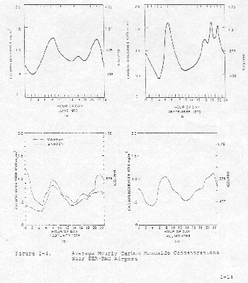
Average diurnal variations in the CO concentrations for the three sampling periods are shown in Figure 2-4. The levels are low and not particularly significant. The only discernible trend is the slight peaking 6-9 a.m. associated with higher activity and the late evening peaking associated with moderate activity light wind, and stable atmospheric conditions.
Analysis of PSAPCA data from May 1972 to April 1973 at the McMicken Heights station shows a hourly maximum of approximately 5 µg/m3 during June and September. The maximum moving 8-hour average was consistent atapproximately 3.5 µg/m3 level during May through September.
Because of the correlation between ESL's measurements during three monitoring periods and data collected by PSAPCA covering an entire year, it is reasonable to assume that the ESL measurements adequately reflect the worst case and average ambient CO levels.
Air samples for hydrocarbon analysis were taken continuously 12 times per hour, 24 hours per day, during June, September, and February. Each sample is buried completely to detect all hydrocarbons, including any naturally
2.4.3 --Continued.
occurring methane gas (CH4). Results are recorded as total hydrocarbons (THC). When unreactive methane gas is separated from the sample, results are recorded as hydrocarbons (HC).
The high 6-9 a.m. average HC concentrations occurred during September. They ranged from approximately 1200 µg/m3 (750 percent of the Federal Primary Standard) to 176 µg/m3 (l10 percent of the Federal Primary Standard) The low 6-9 A.M. averages HC concentrations occurred during February. These ranged from about 380 µg/m3 (240 percent of the Federal Primary Standard) to about 50 µg/m3 (31 percent of the Federal Primary Standard). If all three sampling periods are combined, the 6-9 a.m. average concentrations exceeded the Federal Primary Standard 71 percent of the time.
The mean of the 6-9 a.m. average hydrocarbon levels For all samples was 370 µg/m3 (231 percent of the Federal Primary Standard).
Figure 2-5 shows diurnal variations in hydrocarbon levels. There is a discernible trend similar to an exaggerated version of carbon monoxide diurnal variations (Figure 2-4). Peaking occurs during 6-9 a.m. associated with moderate activity, light wind, and stable atmospheric conditions. Archival data for comparison to the hydrocarbon levels in the Sea-Tac area does not exist.

2.4.3 --Continued.
The levels at the Barden site are particularly significant because they reflect the background level of hydrocarbons in the vicinity of the airport. During the time period the measurements were taken, the wind was primarily from the southwest which would prevent any airport pollutants from reaching the location. Figure 2-5 shows that the background level is very close to the Federal Standard even during the winter periods when hydrocarbon levels are low because of the meteorological conditions.
The high hydrocarbon levels are associated with the “kerosene” odor around the airport. Formation of the aldehydes during the combustion of hydrocarbons will also contribute to the odor associated with the airport. At present, there is no available method for quantifying the odor levels.
Nitrogen dioxide measurements were made at the Marker Station, Golf
course, and Barden sites. Air sampling was performed on a continuous basis
except when calibration or equipment servicing was performed.
In order to estimate the annual averaqe concentration, We have developed seasonal multiplication factors based upon the archival data from McMichen Heights. We assign the average Summer nitrogen dioxide levels a value of 1.0, and compute the multiplication factors as the ratio of the remaining seasonal values to the summer average. Following this procedure the Autumn value is 1.64, Winter is 0.71, and Spring is 0.86. Using these multiplication factors on the Sea-Tac data, we predict nitrogen dioxide averages for the four seasons starting with Summer as 42 µg/m3, 69 µg/m3, 30 µg/m3, and 36 µg/m3. .The annual predicted average for comparison to the Federal Standard would be 44 µg/m3 (.02 ppm) or 44 percent of the standard.
The diurnal trends shown in Figure 2-6 appear to reflect the airport activity with peaking trends during early morning, midday, and late afternoon. Higher levels during late evening hours are caused by stable atmospheric conditions. Archival data from the PSAPCA McMicken station resembles the ESL data, but ESL's data from the Barden site is unique. Because the trend at the Barden site does not follow the airport trend, it would appear that the nitrogen dioxide levels do not result from the airport activity.
Fuel consumption is a major source of nitrogen dioxide and is probably the primary reason the distinct difference between the sites. The Barden site may reflect automobile activity which tends to peak sharply in the morning, but is typically more diffuse in the evening. Also, the prevailing winds were from the southwest during the measurement period; this would prevent airport air pollutants from reaching the site.

Oxidant levels were monitored 24 hours per day during each monitoring
period. In addition, during the peak oxidant period, September, extended
measurements were made.
The maximum hourly oxidant level observed in June was 120 µg/m3 (0.06 ppm) or 75 percent of the Federal Standard of 160 µg/m3 for the 1 hour. During September there were four violations of the Federal Standard on three different days. The highest level observed was 190 µg/m3 or l19 percent of the standard. During the February period, the oxidant levels were nearly zero as expected.
Average oxidant as a function of time is plotted in Figure 2-7 for the June and September periods. These levels cannot be compared to the Federal Standard because they are averaged for all days in the observation period. However, the figures clearly show the expected late afternoon peaks and the higher levels of the autumn season.
Archival oxidant measurements furnished by PSAPCA verify the accuracy of ESL's data. Maximum hourly oxidant levels at the McMicken Heights station during our June observation period was 80 µg/m3 (0.04 ppm), During September their highest hourly value was 120 µg/m3 (0.06 ppm) and their February levels were zero.

2.4.5 --Continued.
Based on the archival data for McMicken for an entire year, and the relationship between the McMicken and ESL data, we expect the oxidant standard to be violated on four or five days per year For a total of 8-10 hours. These occurrences do not represent an immediate problem since the standard is set with an adequate margin of safety, but they do suggest the need to implement any available mitigation measures to reduce hydrocarbons and nitrogen oxides.
Daily 24-hour particulate samples were collected using a high volume
sampler. The geometric mean of all samples was 38 µg/m3
or 49 percent of the annual Federal Standard for the geometric mean. The
highest daily level observed was 112 µg/m3 on a calm day
at the Barden location in February. Both the Marker Station site and the
golf course site reached levels near 100 µg/m3 during
June. These values should be compared to the 24-hour Federal Standard of
260 µg/m3 (40 percent).
Particulate samples collected at the terminal were consistently below those observed at all other sites. Values stapled between 20 and 30 µg/m3 (~10 percent of the standard) for the seven samples taken at the terminal location (Figure 2-8). During September the particulate levels at time golf course site were consistently below those at the Marker station (Figure 2-8).

2.4.6 --Continued.
Because of the prevailing wind direction, takeoffs and landings Were over the Marker Station site. February particulate levels an the Marker Station were not significantly different from September levels, although there was less variation between samples because of rainfall.
The exceptional peak (l14 µg/m3) at the Barden location in February is associated with stagnant atmospheric conditions for nearly 24 hours. Average wind speed during the simple period was 1.5 mph With several lengthy time periods averaging less than 1.0 mph.
Although the above particulate samples are probably representative of the levels expected near Sea-Tac, we also used the Larsen model to estimate the geometric mean and maximum expected value over a one year period. Using this method, the estimated geometric mean is 37 µg/m3 and the maximum expected value is 152 µg/m3. Thus the geometric mean, both observed and calculated, is less than the primary and secondary Federal standards of 75 µg/m3 and 60 µg/m3 respectively.
Archival data from the PSAPCA McMicken Heights Station during the ESL sampling periods does not appear to reflect any airport activity (See Figure 2-8). This is consistent with the fail velocity of particulate, the general wind direction, and the wind speed. These factors tend to move particulate out of the airport region before lateral diffusion to McMicken occurs. During the period from May 1972 through April 1973, the PSAPCA McMicken particulate data had a geometric mean of 42 µg/m3 and a peak of 89 µg/m3. Based on this data and the ESL measurements, it is clear that particulate levels do not exceed Federal Standards at Sea-Tac or in the surrounding communities.
Particulate samples were also analyzed for lead (Pb at the University of California, Davis, cyclotron. Observed lead levels varied between 0.3 µg/m3 and 1.4 µg/m3. The average level was 0.96 µg/m3 For June 1973; and 0.77 µg/m3 for June, September 1973 and February 1974. In the absence of a Federal Standard, these figures can be compared to the California Standard of 1.5 µg/m3 (30 day average). (See Table 2-5.)
Previously, we noted that aircraft operations release large quantities of
carbon monoxide. Automobiles and other ground transportation vehicles also
generate significant quantities of CO. Hence, CO was a natural choice to
measure in the terminal area and surrounding community to determine if
significant levels of pollution existed. This section summarizes the
results of a series of measurements taken within the airport complex and
in the surrounding community.
Table 2-5. Elemental Analysis of Particulate at Sea-Tac Compared to Rural Area in California
| Element | Average Values
Nanograms/CM2 |
|
| Sea-Tac* | Rural Town, CA | |
| Aluminum | 930 | 469 |
| Silicon | 4977 | 6816 |
| Chlorine | 1706 | 1727 |
| Potassium | 916 | 1066 |
| Calcium | 1716 | 2053 |
| Titanium | 220 | ? |
| Iron | 3943 | 4037 |
| Copper | 2732 | 2053 |
| Lead | 3555 + 1670 | 6092 + 2478 |
| Bromine | 563 | 2324 |
*Average flow = 35 ft3/min; Surface Area = 60 in2; Average Concentration of Lead = 0.96 µg/m3 + 0.45 µg/m3
2.4.7 --Continued.
Average carbon monoxide levels in the Sea-Tac terminal area during June 1973 - February, March 1974 are shown in Table 2-6. As would be expected, the higher levels are found in the parking garages, baggage claim areas, and ticketing areas where automobiles are operating nearby. The figures represent hourly averages and are well below the Federal standard of 40 µg/m3 for 1 hour and 10 µq/m3 over 8 hours.
Carbon monoxide levels around the Sea-Tac property tend to be below the terminal levels (Table 2-7). Locations numbered 1 through 5 are closer to aircraft operation and within the airport boundary, and therefore reflect the expected higher CO levels. Again all levels are below the 1-hour and 8-hour standards.
The results discussed above will be used to calibrate the models to be used in predicting future air quality at Sea-Tac. ESL's methodology for predicting air quality is discussed in the following sections.
Table 2-6. Average Daytime Carbon Monoxide Levels Around Sea-Tac Terminal
| CO mg/m3 | Locations | |
| Approximate | Specific | |
| 5.4 | Parking Garage | Lower Level |
| 5.4 | Parking Garage | Top Level |
| 3.8 | Parking Garage | Middle Level |
| 3.4 | S. End | Ticketing |
| 3.4 | S. End | Passenger unload (Street) |
| 4.1 | S. End | Baggage claim |
| 2.9 | S. End | Passenger load (Street) |
| 4.6 | N. End | Baggage Claim |
| 4.5 | N. End | Passenger load (Street) |
| 4.0 | N. End | Ticketing |
| 4.6 | N. End | Passenger unload (Street) |
| 3.2 | C Wing | Inside Begin |
| 3.4 | C Wing | Inside Mid |
| 3.4 | C Wing | Inside End |
| 3.4 | D Concourse | Inside |
| 3.9 | Terminal Lounge | N |
| 4.4 | Terminal Lounge | S |
| 3.1 | B Wing | Inside Begin |
| 2.9 | B Wing | Inside Mid |
| 2.6 | B Wing | Inside End |
| 3.2 | A Concourse | Inside |
| 2.5 | B Wing | Outside Begin |
| 1.8 | B Wing | Outside Mid |
| 1.7 | B Wing | Outside End |
| 2.4 | A Concourse | Outside (NWA Hanger) |
| 2.0 | C Wing | Outside Begin |
| 2.0 | C Wing | Outside Mid |
| 1.9 | C Wing | Outside End |
| 2.0 | D Concourse | Outside |
| 4.8 | Tunnel to | N Satellite |
| 2.2 | Inside | N Satellite |
| 4.6 | Tunnel to | S Satellite |
| 2.4 | Inside | S Satellite |
Table 2-7. Average Daytime CO Levels Sea-Tac Environs
| CO mg/m3 | Grid | Locations
(Approximate) |
| 3.57 | - | WAL Hanger |
| 3.07 | - | Fire Station |
| 4.89 | - | Air Cargo #1 |
| 3.64 | - | UAL Hanger |
| 3.00 | - | Flight Kitchen |
| 3.21 | QR 1718 | Perimeter Road near 518/Airport Fwy |
| 2.46 | QR 1920 | Washington Memorial Park |
| 2.25 | QR 2122 | 171 St./Pacific Hwy (99) |
| 2.82 | QR 2324 | 182nd/Hwy 99 |
| 2.68 | QR 2526 | 188th/Perimeter Road |
| 2.82 | OP 2526 | S188th/34R |
| 2.61 | MN 2526 | S188th/12th |
| 2.54 | MN 2324 | 180th/11 Av S |
| 2.46 | MN 2122 | 172nd 12th |
| 2.39 | MN 1920 | 164th/12th |
| 2.46 | MN 1718 | Renton Three Tree/12 Av S |
| 2.75 | OP 1718 | 154th/20th |
| 2.75 | OP 1516 | Near 518/Extension of 16L |
| 2.39 | QR 1516 | S148th 27th Av |
| 1.93 | ST 1718 | 518/36th |
| 2.54 | ST 1920 | 164th/36th |
| 2.39 | ST 2122 | 172nd/36th |
| 2.46 | ST 2324 | 180th/36th |
| 2.39 | ST 2526 | 188th/36th |
| 2.46 | QR 2728 | 196th/27th |
| 2.32 | OP 2728 | Tynee Valley Golf Club |
| 2.25 | MN 2778 | S196th/Des Moines Way |
| 3.11 | KL 2526 | S188th/8th Av |
| 2.32 | KL 2324 | 180th/8th |
| 2.46 | KL 2122 | 171st/8th |
| 2.46 | KL 1920 | 164th/8th |
| 2.18 | KL 1718 | 156th/8th |
| 2.32 | MN 1516 | 518/Des Moines |
| 2.04 | MN 1314 | 146th/12th |
| 2.46 | OP 1314 | 140th/21st |
| 2.46 | QR 1314 | 140th/28th |
| 2.29 | QR 2930 | 204th/Pacific Hwy |
| 2.29 | OP 2930 | 204th/18th |
| 2.21 | MN 2930 | 204th/12th |
The first step in implementing a model to predict air quality at Sea-Tac
is the compilation of an emission inventory. ESL uses a finite line source
model which requires emissions to be specified along line segments. Each
line segment may be fairly long such as those which would be associated
with approach, landing, takeoff and climb-out; or quite short such as
runway queues and gate parking.
The first step in determining emissions requires a categorization. of
engine types likely to be utilized at the airport. The Cornell
Aeronautical Laboratory (CAL) published emission rates for a large number
of engine types in 1971 at the request of the Environmental Protection
Agency. CAL determined emission factors For three pollutants for a large
number of engine. The results of the CAL study have been supplemented and
published by the EPA (Table 3-1).
To convert the EPA emission factors on Table 3-1 into total emissions, the time each aircraft spends in each operational mode must be specified, operational modes and corresponding modal times are required for taxi-idle prior to takeoff, takeoff, climb-out, approach, and taxi-idle after landing. The emissions according to aircraft type are shown in parentheses in Table 3-1.
Table 3-1. Modal Emission Factor - EPA* (lbs/hr) and Sea-Tac Modal Emissions (lbs)
| Engine & Mode | Carbon Monoxide lbs/hr | Hydrocarbons
lbs/hr |
Nitrogen Oxides
lbs/hr |
Particulate
lbs/hr |
| UT9D
-Taxi-idle -Takeoff -Climbout -Approach Sea-Tac lbs/LTO - Eng. |
102.0 (18.7) 8.8 (0.1) 11.7 (0.43) 32.6 (2.17) 21.4 |
27.3 (5.00) 3.0 (0.135) 2.7 (0.10) 3.0 (0.2) 5.34 |
6.1 (1.12) 720.0 (8.40) 459.0 (16.83) 54.1 (3.61) 29.96 |
2.2 (0.403) 3.8 (0.044) 4.0 (0.147) 2.3 (0.153) 0.747 |
| CF6
-Taxi-idle -Takeoff -Climbout -Approach Sea-Tac lbs/LTO - Eng. |
51.7 (9.48) 6.7 (0.08) 6.6 (0.242) 18.6 (1.24) 11.04 |
15.4 (2.82) 1.3 (0.02) 1.3 (0.05) 1.9 (0.127) 3.02 |
3.6 (0.66) 540.0 (6.30) 333.0 (12.21) 178.0 (11.53) 30.7 |
0.04 (0.007) 0.54 (0.006) 0.54 (0.02) 0.44 (0.03) 0.063 |
| JT8C
-Taxi-idle -Takeoff -Climbout -Approach -Sea-Tac lbs/LTO - Eng. |
109.0 (20.0) 12.3 (0.14) 15.3 (0.14) 39.7 (2.65) 23.35 |
98.6 (18.1) 4.7 (0.05) 4.9 (0.18) 7.8 (0.52) 18.85 |
1.4 (0.26) 148.0 (1.73) 96.2 (3.53) 21.8 (1.45) 6.97 |
0.45 (0.08) 8.3 (0.10) 8.5 (0.31) 8.0 (0.53) 1.02 |
| JT8D
-Taxi-idle -Takeoff -Climbout -Approach Sea-Tac lbs/LTO - Eng. |
33.4 (6.32) 7.5 (0.09) 8.9 (0.33) 18.2 (1.21) 7.75 |
7.0 (1.28) 0.78 (0.009) 0.92 (0.034) 1.75 (0.17) 1.49 |
2.9 (0.53) 198.0 (2.31) 131.0 (4.80) 30.9 (2.06) 9.7 |
0.36 (0.07) 3.7 (0.104) 2.5 (0.095) 1.5 (0.10) 0.305 |
| T56-A7
-Taxi-idle -Takeoff -Climbout -Approach Sea-Tac lbs/LTO - Eng. |
15.3 (2.8) 2.2 (0.02) 3.0 (0.18) 3.7 (0.28) 3.23 |
5.5 (1.2) 0.43 (0.003) 0.48 (0.02) 0.52 (0.04) 1.26 |
2.2 (4.0) 22.9 (0.19) 21.2 (0.88) 7.8 (0.58) 2.05 |
1.6 (0.29) 3.7 (0.03) 3.0 (0.13) 3.0 (0.23) 0.68 |
| TPE332
-Taxi-idle -Takeoff -Climbout -Approach Sea-Tac lbs/LTO - Eng. |
3.5 (0.64) 0.39 (0.002) 0.57 (0.048) 2.6 (0.26) 0.95 |
0.88 (0.16) 0.06 (0.003) 0.05 (0.004) 0.24 (0.024) 0.19 |
0.96 (0.19) 3.64 (0.02) 3.31 (0.28) 1.69 (0.17) 0.65 |
0.3 (0.055) 0.3 (0.004) 0.6 (0.05) 0.6 (0.06) 0.17 |
| CONVENTIONAL 0-200
-Taxi-idle -Takeoff -Climbout -Approach Sea-Tac lbs/LTO - Eng. |
7.5 (1.4) 54.6 (0.27) 54.6 (4.55) 23.8 (2.38) 8.60 |
0.214 (0.04) 0.720 (0.004) 0.720 (0.06) 0.380 (0.04) 0.144 |
0.009 (0.002) 0.259 (0.001) 0.259 (0.02) 0.052 (0.005) 0.08 |
- - - - - |
3.1 --Continued.
Table 3-2 compares the EPA model times to those used in a variety of previous airport studies and those selected for Sea-Tac. Airport configuration and size will play a significant role in the average time assigned to a particular mode, Thus, Dulles (IAD) with aircraft loading and unloading accomplished away from the congested terminal has much shorter taxi-idle times which dramatically reduce emissions. The exceptionally low value for O'Hare is somewhat surprising and is due to low taxi times.
Table 3-2. Average Time Assigned to Aircraft Operating Modes at Verious Airports
| Airports | |||||
| Mode | DCA1 | IAD2 | O'Hare3 | S/T4 | EPA5 |
| Taxi-idle | 11.0 | 5.0 | 7.5 | 7.0 | 19.0 |
| Takeoff | 0.7 | 0.7 | 0.5 | 0.7 | 0.7 |
| Climbout | 1.7 | 1.7 | 2.0 | 2.2 | 2.2 |
| Approach | 4.0 | 4.0 | 3.8 | 4.0 | 4.0 |
| Taxi-idle | 3.4 | 4.0 | 3.9 | 4.0 | 7.0 |
| Total | 20.8 | 15.4 | 17.7 | 17.7 | 32.9 |
3.1 --Continued.
In order to convert the engine emission rates to emission factors, it is necessary to assign the engines to aircraft types, determine the aircraft type distribution for Sea-Tac, end assign the number of engines to each aircraft. Tints is done in Tables 3-3 rind 3-4. It is assumed that the short range aircraft can be represented by the Allison 501D13 engine and that the air taxi general aviation engines can be represented by the Continental 10-570-P and military engines by the JTBD.
Using the EPA emission Factors based on Table 3-1 and 3-2, the total emission tonnage was computed for Sea-Tac in Table 3-5. These figures serve as a useful cross check with other computations for Sea-Tac and with other airports. At the bottom of Table 3-5 figures are presented for Sea-Tac which were obtained from the Puget Sound Air Pollution Control Agency in January 1974. The difference between ESL's calculations using the EPA modal times ("EPA") and the PSAPCA figures is due primarily to differences in aircraft mix. ESL's figures differ from the "EPA" and PSAPCA figures because of the average times, per operating mode reflected in Table 3-2. Sea-Tac modal times in Table 3-2 are based on measurements made at Sea-Tac during 1973 and are considered conservative numbers.
Final Sea-Tac emissions were arrived at by using the operational mode times from Table 3-1. The adjusted figures are 1754 tons/year CO, 1029 tons/year HC, 996 tons/year NOx and 73 tons/year particulate. These figures will be used throughout the remainder of this report to develop emission factors for the model predictions.
Table 3-3. Air Carrier Operations Sea-Tac 1972
| . | 1973
June/July |
1972
113.631 |
Engine
LTOS |
|
| Jumbo | JT9D
(B747) (DC10/L1011) |
5.9% 4.3% |
6704 4886 |
13408 7329 |
| Long Range | JT3D
B707 DC8 |
40.4% |
45907 |
91814 |
| Medium Range | JT8D
B727 DC9 B737 |
31.4% 5.4% 3.3% |
38748 6136 3750 |
58122 6136 3750 |
| . | CJ-805-3A
C880-4A-501-D13 |
. | . | . |
| Short Range | A-501-D13
FH227 L188 |
6.6% |
7500 |
7500 |
| . | . | 100% | 113,631 | 118,056 |
Table 3-4. Total Engine LTSO Sea-Tac Airport 1972
| . | Operations | Regpresentative
Engines |
Engine LTOS |
| I. Air Carrier
-Itinerant -Local |
109,278 4,353 113,631 |
JT9D JT8D JT3D A501-D13 |
188,056 |
| II. Air Taxi
-Itinerant |
17,028 |
JT12 10-520-P |
36,335 |
| III. General
Aviation -Itinerant |
19,307 |
- | - |
| IV. Military
-Itinerant -Local |
1,684 694 152,344 |
N.A. Used JT3D |
4,756 229,150 |
Table 3-5. 1973 Aircraft Emissions at Sea-Tac
| Engine | Engine LTO's | Pollutant | Emission Per LTO (lbs) | Tons/Year | PSAPCA* | ||
| EPA | ESL | EPA | ESL | ||||
| Jumbo
(JT9D) |
13,408 | CO
HC NOx P |
46.9
12.2 31.4 1.3 |
21.4
5.34 30.0 0.75 |
314
82 211 9 |
143
36 201 5 |
- |
| Jumbo
(CF6) |
7,329 | CO
HC NOx P |
23.9
6.87 31.6 0.1 |
11.0
3.0 30.7 0.1 |
88
25 116 0.4 |
40
11 113 0.4 |
- |
| Long Range
(JT3D) |
91,814 | CO
HC NOx P |
50.6
43.5 7.3 1.14 |
23.4
18.9 7.0 1.02 |
2323
1997 335 52 |
1074
867 321 47 |
- |
| Medium Range
(JT8D) |
68,008 | CO
HC NOx P |
16.10
3.25 10.5 0.40 |
7.75
1.50 9.70 0.31 |
547
111 354 13.6 |
264
51 330 10.5 |
- |
| Short Range
(A-501-D13) |
7,500 | CO
HC NOx P |
7.0
2.7 3.3 6.0 |
7.0
2.7 3.3 6.0 |
26
10 12 23 |
26
10 7 4 |
- |
| Air Taxi And General Aviation
(10-520-P) |
36,335 | CO
HC NOx P |
8.3
0.5 0.4 0.2 |
8.3
0.5 0.4 0.2 |
151
9 7 4 |
1515
9 7 4 |
- |
| Military
(JT3D) |
4,756 | CO
HC NOx P |
50.6
43.5 7.3 9.4 |
50.6
43.5 7.3 0.4 |
120
103 17 2.7 |
56
45 17 2.4 |
- |
| Total Tons/Year
|
CO
HC NOx |
3569
2337 1052 105 |
1754
1029 996 73 |
3133
2133 890 86 |
|||
3.1 --Continued.
Table 3-6 compares the ESL predicted annual emissions to comparable figures developed by other groups for several airports. Estimates for the same airport differ dramatically depending on the source even though some estimates are for the same year. The apparent uncertainty in total emissions emphasizes the importance of making air quality measurements near the airport to calibrate the base year model predictions.
Fuel venting is a potential source of hydrocarbon emissions by aircraft.
At engine shutdown, drainage from the Fuel manifold is collected in a
drain tank in each engine nacelle. At start up, a little more fuel is
added to this quantity before. the dump valve is closed. After takeoff the
collected fuel is purged by the ram air pressure. Average HC loss due to
fuel venting based 'upon 160 takeoffs per day would amount to
approximately 600 lbs. per day. Most of this would be lost at air altitude
of perhaps 600 meters which, according to a precious report, would produce
ground level concentrations of no more than 10-15 µg/m3.
Operation of auxiliary power units is another source of aircraft emissions. If 1 hour of operation per LTO is assumed, then based on available emission factors an additional 94 tons of CO, 8 tons of NOx, and 9 tons of hydrocarbons will be emitted annually.
Table 3-6. Aircraft Emissions in Tons at Sea-Tac and Other Airports
| Airport | CO | HC | NOx | P | Year |
| Sea-Tac | 1,848
|
1,038
|
1,004
|
73
|
1972-1973
|
| Los Angeles1 | 10,9751 | 10,725 | 1,105 | 2,250 | 1970 |
| Dulles2 | 659 | 427 | 410 | 314 | 1973 |
| D.C. National2 | 1,018 | 164 | 1,147 | 1,026 | 1973 |
| O'Hare3 | 14,740 | 9,580 | 3,760 | 900 | 1970 |
| Kennedy3 | 12,590 | 9,490 | 2,580 | 570 | 1970 |
| National3 | 2,410 | 610 | 820 | 231 | 1970 |
| Los Angeles3 | 16,030 | 12,570 | 3,060 | 570 | 1970 |
1"Study of Jet Aircraft Emissions and Air Quality in the Vicinity of Los Angeles International Airport," Los Angeles County Air Pollution Control District, April 1971.
2Monitoring and Modeling of Airport Air Pollution, D.M. Rote, et. al., International Conference on Transportation and the Environment, 1972.
3"Draft Environmental impact Statement for Policy Changes on the Role of Washington National Airport and Dulles International Airport," Office of Environmental Quality, AIQ-30 Dept. of Transportation, FAA.
3.2 --Continued.
Maintenance operations are potential sources of air pollution, but are not considered significant compared to the aircraft operations and motor vehicle sources.
3.3 --Automobile Emissions.
Automobile traffic along the roads adjacent to airports and in the terminal parking area is a major source of air pollution near airports. Because it is desirable to relate the automobile emissions to the airport traffic, it is customary to assume a certain number of vehicle operations for each passenger arrival or departure, and an additional factor for employee automobile traffic,
Based on (1) passenger traffic of 4,788,962, (2) 7,000 employees in 1972, and (3) 1.24 passengers per car; approximately 16,000 vehicles per day are predicted on the average. This compares to the 20,000 vehicles per day supplied by the Sea-Tac Communities Plan Study Group. Some of the difference may be related to air freight and postal activities.
Vehicle emissions associated with the airport occur throughout King Country. Since this study assesses that contribution in the environs of the airport, travel near the airport only is considered. Specifically, it is assumed that the 20,000 vehicles drive 2.0 miles at 45 MPH and 0.25 miles at 15 MPH. Based on these figures, automobiles should add approximately 669 tons of CO, 107 tons of hydrocarbons, 126 tons of nitrogen oxides, 11 tons of particulate, and 1.1 tons of lead to the Sea-Tac ambient air during an average year (Table 3-7). Additional automobile emissions occur within time airport boundary along S. 188th St., HWY 518, HWY 99, S. 154 St., and others. These emissions are a source of air pollution in the area, but are not considered as part of the Sea-Tac impact in this report.
Average annual emissions near Sea-Tac and those associated with aircraft operations and access vehicles are summarized in Table 3-8. Clearly, aircraft operations are the major source of air pollutants near Sea-Tac, particularly hydrocarbons, nitrogen oxides and particulate. The determination of whether these emissions will cause significant air pollution requires a sophisticated mathematical model which is discussed in Section 4 of this report.
The heating plants of all buildings, air conditioning facilities, flight
kitchens, and even the hot water boilers consume natural gas and fuel.
Combustion of the fuel will release pollutants including carbon monoxide,
hydrocarbons, nitrogen oxides, and particulates.
Table 3-7. 1973 Vehicular Emissions at Sea-Tac
| Pollutant | Emission Factor | Speed Factor
(15 MPH) |
Speed Factor
(45 MPH) |
Emissions
(gms/Auto) |
Emissions
Tons/Year |
| Carbon Monoxide | 62 | 1.25 | 0.515 | 83.24 | 669 |
| Hydrocarbons | 6.1+2.0 | 1.17 | 0.58 | 13.26 | 107 |
| Nitrogen Oxides | 5.4 | 0.95 | 1.33 | 15.65 | 126 |
| Particulate | 0.58 | 1.00 | 1.00 | 1.31 | 11 |
| Lead | 0.06 | 1.00 | 1.00 | 0.14 | 1.1 |
*Compilation of Air Pollutant Emissions Factors, Second Edition U.S. Environmental Protection Agency, Revised September 1973.
Table 3-8. Annual Emissions at Sea-Tac Due to Aircraft and Motor Vehicles (Tons/Year)
| Pollutant/Source | CO | HC | NOx | P | Pb |
| Aircraft | 1,754 | 1,029 | 995 | 73 | ? |
| Motor Vehicles | 669 | 107 | 126 | 11 | 1.1 |
| Total | 2,423 | 1,136 | 1,122 | 83 | 1.1 |
3.4 --Continued
Emission factors have been developed by the Environmental Protection Agency for fuel oil and natural gas combustion as shown in Table 3-9. Based on this table, fuel combustion may affect nitrogen oxide and particulate levels in the Sea-Tac environs.
Fuel combustion at Sea-Tac cannot be predicted reliably because of the potential for serious fuel shortages in the future. natural gas service is expected to be disrupted frequently during 1974 and future years. The long term effect probably will reduce total fuel consumption and increase the proportion of fuel oil used.
Table 3-9. Emission Factors for Fuel Oil and Natural Gas Combustion*
| Pollutant | Fuel Oil (Residual)
Lbs/1,000 Gallons |
Natural Gas
Lbs/1,000,000 ft3 |
| Carbon Monoxide
Hydrocarbons Nitrogen Oxides Particulates |
4
3 60 23 |
20
8 (CH4) 100 19 |
*Compilation of Air Pollution Emission Factors EPA #AP-42, April 1973.
Table 3-10. Total Emissions for Fuel Oil and Natural Gas Combustion
| Pollutants | Emissions Fuel Oil
(Tons/Year) |
Emissions Natural Gas
(Tons/Year) |
| Carbon Monoxide
Hydrocarbons Nitrogen Oxides Particulates |
0.33
0.25 4.92 1.89 |
3.57
---- 17.86 3.39 |
3.4 --Continued.
For purposes of estimating the impact on air quality, the fuel consumption estimates made prior to the 1973 "Energy Crisis" were used. Natural gas consumption was estimated to be 3.3 million therms and fuel oil consumption at 164,000 gallons.
Total emissions on an annual basis are shown in Table 3-10. With the possible exception of particulate, these emissions do not constitute a significant proportion of aircraft emissions (Table 3-5). Particulate emissions are 7 percent of those associated with aircraft emissions and will contribute to overall particulate levels.
Loss of vapor due to evaporation from storage tanks during daily
temperature fluctuations and the displacement when the tanks are filled is
another potential source of hydrocarbons.
Fuel spills during refueling of aircraft and ground service vehicles will evaporate into the ambient air. Normally, these spills will be washed away due to fire hazards. Fuel spillage , therefore, will generally contribute to water pollution rather than air pollution.
Losses resulting from the displacement of vapor during refueling are referred to as working losses, whereas evaporative losses are referred to as breathing losses. Both sources can be controlled with vapor recovery systems.
Aircraft fuel at Sea-Tac is stored in eight floating roof tanks with a total capacity of 580,000 barrels or 24,360,000 gallons. Total fuel deliveries are approaching six million barrels per year.
A floating roof tank is an effective device for minimizing both breathing and working losses. The basic design virtually eliminates vapor space resulting in low emissions due to breathing, filling, and emptying. Based on this design we have assumed that there are no breathing losses of significance from the storage tanks at Sea-Tac.
Refueling of ground service vehicles and aircraft will produce working
losses. The vapor emissions from aircraft refueling can be seen as density
waves appearing above the wing filling ports.
An empirical equation for estimating working losses due to refueling was developed by the American Petroleum Institute Argonne converted the API equation into working less per 1,000 gallons of fuel pumped. The final figures were 0.55 lbs/1,000 gallons for aircraft fuel and 3.63 lbs/1,000 gallons for around service vehicles.
Total fuel deliveries of jet fuel were estimated to be 239 million gallons at Sea-Tac. Ground service vehicles were assumed to require 330,000 gallons of gasoline. Taken together, refueling should produce approximately 66 tons per year of additional hydrocarbons. This is about 6 percent of the estimated aircraft hydrocarbon emissions for 1973.
The figure of 66 tons will be increased in proportion to the increase in aircraft operations to predict losses in the future.
Motorized vehicles associated with servicing aircraft in the gate areas
contribute to the air pollutant emissions at Sea-Tac. Included in this
category are tractors, belt loaders, food trucks, fuel trucks, etc.
Computation of emissions from these vehicles is difficult and subject to uncertainty, since emission characteristics have not been measured. Moreover, utilization factors are uncertain and the maintenance programs vary among airlines.
The procedure used by Argonne in their EPA report involved estimating utilization times for each service vehicle as a function of aircraft type, adopting emission factors for heavy duty trucks, estimating the average miles/gallon for each vehicle, and assigning average speeds for operational use. In addition, they assumed that the Federal automotive emission controls would be applied to ground service vehicles.
Because of the above uncertainties, in this report we have simplified the Argonne approach by relating the ground based emissions to the fuel consumption of these vehicles. To do this we assumed that the vehicles average 10 MPH and get 6 miles per gallon. These factors are combined with the EPA automobile emission factors to yield emissions in grams/gallon (Table 6-9). based on this approach, we predict 207 tons carbon monoxide, 27 tons hydrocarbons, 11 tons nitrogen oxides and 1 ton of particulate for 1973 for 330,000 gallons of fuel.
In this section we have compiled a list of pollution sources, I.e., an emission inventory at Sea-Tac. The next step in establishing the air quality impact of these emissions is to develop a model for predicting the dispersion of the pollutants into the ambient atmosphere. ESL's model is discussed in the next section.
ESL used a finite line source model to predict the air quality near the
Sea-Tac Airport. The entire emission inventory previously discussed was
assigned to one or more line segments. Some sources such as the runways
and taxiways were adequately represented by a single finite line. Others,
such as the parking garage, were represented by multiple line segments at
various heights above the ground.
The meteorological inputs to the finite line source model are wind speed, wind direction, height of inversion base, and turbulence which may be specified in terms of the Pasquill class. The source inputs are the source height, endpoints, and emission strength. An inclined source, such as the climb-out Path, is approximated by a series of horizontal segments resembling a staircase.
The advantages of using a finite line source instead of finite set of points to approximate a linear intended source are:
a. A more accurate representation is obtained
b. Fewer data inputs are required
c. Computation time is reduced
d. A greater number of sources may be considered simultaneously
e. Less user time is required to assemble the data inputs for the model.
The model for finite line sources is derived by the method of
superposition from the Gaussian formula for a continuous point source
which states that the pollutants are normally distributed in the crosswind
and vertical directions provided there are no absorbing or reflecting
surfaces present. In order to account for reflections from the ground
plane or inversion base, the image of the source in the reflecting plane
is assumed to he a virtual source whose plume is combined with that from
the actual source to determine emission levels. To account for multiple
reflections, for example, from the ground plane to inversion base and back
to the ground plane, the standard method of introducing multiple images
(images of images) is employed.
Consider a contini;ous point source emitting an unreactive gas above a non-reflecting, non-absorbing ground plane. The mean concentration predicted by the Gaussian plume formula at receptor (x, y, z) is:

4.1 --Continued.
where x is the downwind distance from the source, y is the crosswind distance from the plane centerline, z is the elevation of the receptor, h is the elevation of the source, Q is the emission rate of the source, and u is the magnitude of the mean wind velocity.
Using the empirical formulas for the standard deviation of lateral wind direction of the relative concentration distribution and the standard deviation of horizontal wind direction of the relative concentration distribution, derived by the National Reactor Testing Station at Idaho Falls, namely,

4.1 --Continued
the dispersal model for a finite line source may be obtained from equation (1) by integration.
In order to conveniently formulate the dispersal model equations, the coordinate system illustrated in Figure 4-1 is introduced. The origin of the coordinate system is taken to be the ground point directly below the receptor P, and the positive x-axis is taken to extend in the direction from which the mean wind blows. We vertical axis through the origin is

4.1 --Continued.
defined to be the positive z-axis, and the endpoints of the finite line source are denoted by A, B, where by convention, A is taken to be the point furthest downwind. The coordinates of A, B are denoted by (xA, yA, h), (xB, yB, h) where h is the height of the line source above the ground plane. The variable xA = maximum (0, xA},
![]() is the angle between the line source and the mean wind velocity, D is the
ground distance between the receptor and the infinite line collinear with
AB, and (0, 0, zO) are the coordinates of the receptor P.
is the angle between the line source and the mean wind velocity, D is the
ground distance between the receptor and the infinite line collinear with
AB, and (0, 0, zO) are the coordinates of the receptor P.
(NPC Editor's Note: Because of the complexity of putting the above a-ish fishy symbol in, we are henceforth going to put in a "@" as a substitute. We apologize for any inconvenience this may bring about)
In the absence of an inversion layer, the concentration X(P), at the receptor, is obtained from the equation
.gif)
and the variables on the right hand side of the equation are defined as follows:
.gif)

Equation (2) is the general formula for concentration whenever the wind is not normal to AB and either D > 0 or z0 does not = L. The special cases when D does not = 0 and z0 = h or the wind is normal to AB and divided into three subcases, and similar formulas are derived by integration.
In the event of an inversion base at a height H, equation (2) must be augmented to include simple and multiple reflections from both the inversion layer and the ground plane. The number of reflection terms will depend upon the distance of the receptor from the source, turbulence, and the height of the inversion layer. More precisely, let xo satisfy 2.15 @(xo) = H; then equation (2) will apply to all receptors whose downwind distance from all contributing source points is less than xo. A source point is considered to contribute to the concentration at a receptor if the receptor lies within an angle 3.5 @(theta) downwind of the source (see Figure 4-2). The angle 3.5 @(theta) was chosen to correspond with the horizontal boundary of the plume emanating from a source point, i.e., those points in the horizontal plane through the plume centerline where concentrations are ten percent of the centerline concentrations. In the general case, equation (2) becomes

and I, Si are defined as follows:

4.1 --Continued.
I = smallest integer which is greater than or equal to
(dMAX)/(xo)
dMAX, measured along mean wind direction, is the maximum upwind distance to any contributing source point.
S1 = (zo-h), S2 = (zo+h)
Si = z0 - 2M(-1)r+1 * (H+f(r)h), i > 3
where r is the remainder when i-2 is divided by 4, M is the smallest integer >= ((i-2)/4), and f(r) is defined by
f(0) = -1
f(1) = -1
f(2) = 1
f(3) = 1
The special cases, (1) D = 0 and zO = h, and (2) normal wind, are similarly generalized for reflections off the inversion layer.
To apply the model, the location of the all receptors and finite sources
are specified in terms of a fixed convenient coordinate system.
Specifically, the ground coordinates and height are indicated for each
receptor and line source endpoint. To calculate the concentration at a
particular receptor, a linear transformation and translation is performed
which transforms the input coordinates of the line sources into the
coordinate system appropriate for application of the above concentration
formulas. The new coordinate system has its origin at the ground point
below the receptor, and its positive x-axis points in the direction from
which the mean wind blows.) The contribution of each source to the
concentration at the receptor is calculated, and all the component
concentrations are summed to determine the total pollutant level.
The mathematical model discussed in the previous section predicts
pollutant concentration at several hundred receptors around the airport. A
set of calculations is made for each wind direction. Aircraft sources are
positioned according to whether landings and takeoffs are north to south
or south to north.
Air quality predictions are made for "worst case and “most probable” conditions. Average or "most probable" conditions were defined as Pasquiil turbulence classification B, 5 mile per hour wind speed, and average airline activity. "Worst case" conditions were defined as 2 mile per hour wind speed, Pasquill turbulence classification D, and peak airline activity.
Finally, the maximum Pollutant concentrations at each receptor are used to construct the "worst case" isopleths. Average or "most probable" isopleths are constructed from the weighted average concentration at each receptor. The weighting factor is the frequency that a given wind direction is observed at Sea-Tac.
Given the conditions outlined above, the proper interpretation of the isopleths can be expressed in the following manner: the worst case isopleth for a given pollutant represents the highest levels anal would be expected at a given location over a 1-year period for the specified time interval. These isopleths do not represent a condition that would exist simultaneously over the area covered by the isopleths. This is because a northerly wind with stable atmospheric conditions will not produce high pollutant concentrations north of the airport. Another way to express this condition is to consider the worst case isopleths as defining the maximum area that could be impacted by the airport. If any isopleth is higher than the corresponding federal standard, that area is expected to experience violations of the standard sometime during the year.
Similarly, tie average isopleths represent the expected pollutant concentrations at a given location for the indicated time period. Again, the wind direction must be favorable unless the standard is for one year.
Predicted carbon monoxide levels are well below the Federal Standards of
10 µq/m3 for 8 hours and 40 µg/m3 for I
hour (Figures 5-1 and 5-2). Typical values are 1-3 µg/m3
and the worst case 1 hour figures are not expected to go above 6-8 µg/m3.
These are no known adverse health effects associated with these levels.
The predicted hydrocarbon levels near Sea-Tac exceed the Federal standard
over large areas (Figures 5-3 and 5-4). Part of this is caused by the
generally high backqround levels which tend to be near the standard
itself. The rest is due to the proportionately higher hydrocarbon
emissions of aircraft, Hydrocarbon emissions are approximately 60 percent
of carbon monoxide emissions, and the very low hydrocarbon standard is
easily violated.
Hydrocarbon standards are not set at 160 µg/m3 because of their known adverse health effects. Rather, as was discussed in Section 1 of this document, the HC standard is set to keep oxidant levels in an area from creating a health hazard, The significance of HC on oxidant formation is discussed below.
Nitric Oxide (NO) is eventually converted to nitrogen dioxide (NO2)
in the atmosphere, The exact mechanism and time frame for accomplishing
this is not completely understood, As a result it is common practice to
measure the total amount of NO and NO2 by oxidizing the NO to
NO2 and detecting NO2. The total amount present is
recorded as NOx. Federal standards apply only to NO2
(100 µg/m3, annual average), and hence NOx
represents a conservative estimate of local NO2 levels. Figure
5-5 depicts the predicted 1973 annual average NOx
concentrations, Because the standard is specified as an annual average, "worst
case" conditions are not meaningful. The only place where standard is
likely to be exceeded is the runway area itself.
No adverse health effects are expected from the high levels of NOx on the runway itself. In this area most of the NOx is probably in the form of NO, and personnel are not exposed to the high levels.
EPA, emission factors for particulate which were published in April of
1973 are too small to yield detectable particulate levels around Sea-Tac.
No explanation was given in the new report for dramatically reducing the emission factors for particulate. For example, in the February 1972 report, the JT9D engine was listed as producing 10 pounds of particulate per LTO (landing- takeoff cycle) whereas the April 1973 report listed the JT9D at 1.30 pounds. Similarly, the 1972 figure for the JT3D engine was 8 pounds per LTO, and 7 pounds per LTO for the JTBD engine; the corresponding 1973 figures were 1.21 pounds/LTO and 0.41 pounds/LTO, respectively.
Based om the EPA model times, this represents an average reduction of 88 percent between February 1972 and April 1973. Unless these changes are erroneous, it must be concluded that aircraft operations do not generate significant (less than 25 µg/m3) 1evels of particulate near Sea-Tac.
However this condition does not seem justifiable since even the casual observer can see the heavy particulate emissions of departing aircraft and the moderate emissions from arriving aircraft. Accordingly, we have multiplied the emissions by a factor of four in order to bring the model predictions into line with the observed particulate levels at Sea-Tac.
Predicted annual particulate levels based on adjusted emissions are shown. in Figure 5-6. The numbers on the isopleths represent the geometric mean which must be calculated from the model predicted average particulate Level. To do this we assume that the model average is from a distribution with the same standard geometric deviation as the particulate samples collected at Sea-Tac (l.62). The geometric mean is then calculated using the formula:
Mg = X / (Sg)(1/2 ln*Sg)
Where
X = arithmetic mean
Mg = geometric mean
Sg standard geometric deviation
ln = the natural logarithm to the base
Using the value of Sg = 1.62, the geometric mean big is 0.89 times the arithmetic average. Thus, the geometric mean is slightly less than the average value predicted.
Even with the adjusted emission factors the predicted geometric mean is below the primary Federal Standard (75 µg/m3) and the secondary Federal Standard (60 µg/m3) (see Figure 5-6).
Worst case conditions using the adjusted emission factors are shown in Figure 5-7. These 24-hour average levels should be compared to the Federal primary Standard (260 µg/m3) and the corresponding secondary Federal Standard (150 µg/m3). Again, neither standard should be violated at or near Sea-Tac.
The aviation gasoline used by aircraft piston engines contains tetraethyl lead and halogenated scavenging agents in quantities similar to those in automotive fuel. Lead compounds in the form of particulate matter are formed during the decomposition of these additives. Piston engine aircraft will not generate appreciable amounts o± lead at Sea-Tac, and the Environmental Protection Agency has not set any federal standard for lead.
Photochemical oxidant is not a pollutant emitted into the atmosphere by
transportation sources. (A more complete discussion of the processes
leading to the formation of oxidant was given in the first section of this
report.) Essentially hydrocarbons, nitrogen oxides, and sunlight interact
to form ozone and other oxidants. Based on Figures 1-2 and 1-3, high early
morning hydrocarbon levels and/or high levels of nitrogen oxides are
associated with high oxidant levels later in the day. The high levels
referred to in these figures correspond generally to measurements made
over a large area such as an air basin or the Puget Sound Air Pollution
Control District. Thus, the high hydrocarbon levels observed at Sea-Tac
are not expected to he associated with high oxidant level at Sea-Tac
unless background level of hydrocarbons and/or nitrogen dioxide are also
high. At Sea-Tac the highest oxidant level was 190 µg/m3
(10 ppm), at Des Moines the highest level was 80 µg/m3
(0.04 ppm), and McMicken Heights recorded a high of 215 µg/m3
(0.11 ppm). The 1-hour oxidant standard (160 µg/m3, 0.08
ppm) was exceeded 14 times during August and September at the McMicken
Heights site. Thus, oxidant levels recorded at McMicken Heights simply
that hydrocarbon and/or nitrogen dioxide background levels are generally
high in the area. Accordingly, it would be desirable to reduce hydrocarbon
emissions in the area as a means of controlling oxidant formation.
The air quality in the future near Sea-Tac will depend upon the increase
or decrease in aircraft operations, the aircraft mix, ambient air quality,
and the effectiveness of air pollution emission standards for aircraft
engines. Each of these factors will have an impact on air quality and is
briefly discussed below.
The Environmental Protection Agency has set final air pollution emission
standards for aircraft engines, proposed an engine retrofit program, and
announced a trial program of aircraft ground operations control. In
addition, fuel venting is prohibited for the T2, T3, and T4 engines after
January 1, 1974, and for all T1 and P2 engines after January 1, 1975. The
T2, T3, and T4 engines represent more than 75 percent of current
operations.
Emissions of carbon monoxide, smoke (particulate), hydrocarbons, and nitrogen oxides will be limited by the new standards; and all types of aircraft will be affected (Table 6-1). If these figures are attained, average reductions would amount to 73 percent for carbon monoxide, 80 percent for hydrocarbons, and 43 percent for nitrogen oxides for turbine engines (T2, T3, T4).
Additional standards proposed for 1981 would require further reductions in hydrocarbons and carbon monoxide, but would not change nitrogen oxides (Table 6-1). These standards would aptly only to the turbine (T2) class of engines over
Table 6-1. Proposed Aircraft Emission Standards
| 1979 New Manufactured | 1981 New Certified | ||||||
| Fuel VentingProhibited | HC* | CO* | NOx* | HC* | CO* | NOx* | |
| Turbine (T1)
Piston (P2) Turbine (T2) Turbine (T3) Turbine (T4) Piston (P1)** APU |
January 1, 1975
January 1, 1975 January 1, 1974 January 1, 1974 January 1, 1974 |
1.6
4.9 0.8 0.8 0.8 1.9 0.4 |
9.4
26.8 4.3 4.3 4.3 42.0 5.0 |
3.7
12.9 3.0 3.0 3.0 1.5 3.0 |
0.4
|
3.0
|
3.0
|
*Pounds/1000 x rated power/cycle-piston engines; pounds/1000 hp-hr of
power output-auxilary power unit; pounds/1000 pound-thrust
hr/cycle-aircraft engine.
T1-Turbofan or turbojet engines of rated power less than 8000 pounds
thrust. (Aircraft examples: business and private jets such as Lear Jet,
Grumman Gulfstream, Lockheed Jetstar and Cessna Citation.)
T2-Turbofan or turbojet engines, except classes T3 and T4, of 8000
pounds or greater. (Aircraft examples: Boeing 747, Lockheed L1011, and
DC-10.)
T3-All JT3D model engines (Aircraft examples: Boeing 707, DC-8.)
T4-All JT8D model engines (Aircraft examples: Boeing 727, 737, DC-9.)
P1-All piston engines, except radials. (Aircraft examples: All piston
engine planes ranging from the Cessna 150 of Piper Cherokee 140 to the
Beechcraft Queen Air.)
P2-All turboprop engines. (Aircraft examples: Lockheed Electra,
Fairchild F27, and Convair 540.)
F27, and Convair 540.)
APU-Auxiliary Power Unit-Any engine on the plane exlusive of
propulsion engines. APU's used to operate on-board power systems when
propulsion engine not operating
**Effective for engine built after December 31, 1979.
| Engine | Effect of Emission Standards | ||
| CO | Existing
HC |
NOx | |
| JT3D (T3)
JT8D (T4) JT9D (T2) % Reduction Jt3D (T3) JT8D (T4) JT9D (T2) AVG % Reduction |
30.191
12.488 11.316 86 67 66 73 |
25.88
2.794 2.950 92 71 78 80 |
4.335
4.977 7.581 31 39 60 43 |
6.1 --Continued.
8,000 pounds thrust. At present it is not known if any research effort is underway to accomplish the 1981emission goals.
EPA has also proposed requiring a retrofit on all pre-1979 gas turbine engines of class T2 and a rated power exceeding 29,000 pounds. The proposed change, scheduled for completion by January 1, 1983 would bring all class T2 engines to 1979 standards. At the present time, there is strong opposition to the proposed retrofit, and implementation is uncertain.
Given the time frame for emission standards and the length of time required for engines introduced after 1979 to enter the general aircraft population, emission rates are not expected to change at all by 1978, very little by 1983, and moderately by 1993. Other factors such as vehicle mix and ground controls can have a significant impact by 1978 and 1983 and are discussed in Section 7.
Peat, Marwick, Mitchell and Co. furnished Sea-Tac air traffic forecasts
and aircraft mix for air carrier operations (Tables 6-2, 6-3) for the
years 1978, 1983, and 1993.
These projections were used to develop engine LTOS for each year as shown in Table 6-4. Environmental Protection Agency emission factors (Table 3-1) shown here as Table 6-5 were used to calculate predicted Sea-Tac emissions for 1973, 1978, 1933, a-zd1993 ail aircraft type (Table 6-6).
Table 6-2. Sea-Tac Air Traffic Forecasts 1978, 1983, 1993
| Type | 1978 | 1983 | 1993 |
| I. Air Carrier
-Itinerant -Local II. Air Taxi Scheduled III. General Aviation IV. Military Total Operations: Total LTOs |
125,000
121,000 4,000 20,000 25,000 2,000 172,000 86,000 |
146,000
142,000 4,000 24,000 30,000 2,000 202,000 101,000 |
180,000
176,000 4,000 32,000 40,000 2,000 254,000 127,000 |
Table 6-3. Sea-Tac Aircraft Mix* 1978, 1983, 1993
| Aircraft Class | Representative Engine | %1978 | %1983 | %1993 |
| Jumbo
747 DC-10-L1011 |
JT9D CF6 |
5.5 14.8 |
5.1 22.0 |
4.9 40.2 |
| Long Range
707: CD-8 |
JT3D |
27.3 |
15.4 |
- |
| Medium Range
727, 7x7 737 DC-9 |
JT8D JT8D |
40.4 9.3 |
47.7 7.5 |
54.9 - |
| Air Carrier Turboprop
L188 F-27/C-640 |
501-D13 501-D15 |
- 2.7 |
- 23.0 |
- - |
*Peat, Marwick, Mitchell and CO., 6 June 1974.
Table 6-4. Sea-Tac Engine LTOs* 1978, 1983, 1993
| Aircraft | Engs. | 1978 | 1983 | 1993 |
| Jumbo
747 DC10-L1011 |
4 3 |
13,750 27,750 |
14,892 48,180 |
17,640 108,540 |
| Long Range
707, DDC-8 |
4 |
68,250 |
44,968 |
- |
| Medium Range
727, 7x7 737, DC9 |
3 2 |
75,750 11,625 |
104,463 10,950 |
148,230 - |
| Aircraft Carrier Turbo
F-27/C-640 |
2 |
3,375 |
3,358 |
- |
| SUB-TOTAL ENGINE LTOs | - | 200,500 | 226,811 | 274,410 |
| Air Taxi
General Aviation Military |
2
1.5 4 |
20,000
18,750 4,000 |
24,000
22,500 4,000 |
32,000
30,000 4,000 |
| Total Engine LTOs | - | 243,250 | 277,311 | 340,410 |
*LTO = Descent from 3,500 feet, landing taxi, idle, idle, taxi, takeoff, climbout, climbout to 3,500 feet.
Table 6-5. Modal Emission Factors - EPA* (lbs/hr) and Sea-Tac Modal Emissions (lbs)
| Engine & Mode | Carbon Monoxide
lb/hr |
Hydrocarbons
lb/hr |
Nitrogen Oxides
lb/hr |
Particulate
lb/hr |
| JT9D
Taxi-idle Takeoff Climbout Approach Sea-Tac lbs/LTO - Eng. |
102.0 (18.7) 8.3 (0.1) 11.7 (0.43) 32.6 (2.17) 21.4 |
27.3 (5.00) 3.0 (0.135) 2.7 (0.10) 3.0 (0.2) 5.34 |
6.1 (1.12) 720.0 (8.40) 459.0 (16.83) 54.1 (0.01) 29.95 |
2.2 (0.403) 3.8 (0.044) 4.0 (0.247) 2.3 (0.145) 0.747 |
| CF6
Taxi-idle Takeoff Climbout Approach Sea-Tac lbs/LTO - Eng. |
51.7 (9.43) 6.7 (0.08) 6.6 (0.242) 18.6 (1.24) 11.04 |
15.4 (2.82) 1.3 (0.02) 1.3 (0.05) 1.9 (0.127) 3.02 |
3.6 (0.66) 540.0 (6.30) 333.0 (12.21) 173.0 (11.53) 30.7 |
0.04 (0.007) 0.54 (0.006) 0.54 (0.02) 0.44 (0.03) 0.063 |
| JT3D
Taxi-idle Takeoff Climbout Approach Sea-Tac lbs/LTO - Eng. |
109.0 (20.0) 12.3 (0.14) 15.3 (0.56) 39.7 (2.65) 23.35 |
98.6 (18.1) 4.7 (0.05) 4.9 (0.18) 7.8 (0.52) 18.85 |
1.4 (0.25) 148.0 (1.73) 96.2 (3.53) 21.8 (1.45) 6.97 |
0.45 (0.08) 8.3 (0.10) 8.5 (0.31) 8.0 (0.53) 1.02 |
| JT8D
Taxi-idle Takeoff Climbout Approach Sea-Tac lbs/LTO - Eng. |
33.4 (6.12) 7.5 (0.09) 3.9 (0.33) 18.2 (1.21) 7.75 |
7.0 (1.28) 0.78 (0.009) 0.92 (0.034) 1.75 (0.17) 1.49 |
2.9 (0.53) 198.0 (2.31) 131.0 (4.80) 30.9 (2.06) 9.7 |
0.36 (0.066) 3.7 (0.043) 2.6 (0.095) 1.5 (0.100) 0.304 |
| T56-A7
Taxi-idle Takeoff Climbout Approach Sea-Tac lbs/LTO - Eng. |
15.3 (2.8) 2.2 (0.02) 3.0 (0.13) 3.7 (0.28) 3.23 |
6.5 (1.2) 0.43 (0.003) 0.48 (0.02) 0.52 (0.04) 1.26 |
2.2 (4.0) 22.9 (0.19) 21.2 (0.88) 7.8 (0.58) 2.05 |
1.5 (0.29) 3.7 (0.03) 3.0 (0.13) 3.0 (0.23) 0.68 |
| TPE331
Taxi-idle Takeoff Climbout Approach Sea-Tac lbs/LTO - Eng. |
3.5 (0.64) 0.39 (0.002) 0.57 (0.048) 2.6 (0.26) 0.95 |
0.88 (0.16) 0.06 (0.003) 0.05 (0.004) 0.24 (0.024) 0.19 |
0.96 (0.18) 3.64 (0.02) 3.31 (0.28) 1.69 (0.17) 0.65 |
0.3 (0.055) 0.8 (0.004) 0.6 (0.05) 0.6 (0.06) 0.17 |
| Continental 0-200
Taxi-idle Takeoff Climbout Approach Sea-Tac lbs/LTO - Eng. |
7.5 (1.4) 54.6 (0.27) 54.6 (4.55) 23.8 (2.33) 8.60 |
0.214 (0.04) 0.720 (0.004) 0.720 (0.06) 0.380 (0.04) 0.144 |
0.009 (0.002) 0.259 (0.001) 0.259 (0.02) 0.052 (0.005) 0.01 |
- - - - |
*Compilation of Air Pollution Emission Factors, 2nd Edition U.S. EPA April 1973
Table 6-6. Predicted Sea-Tac Emissions (Tons/Yr)
| Engine-Pollution/Year | 1973 | 1978 | 1983 | 1993 |
| JT9D - Jumbo
Carbon Monoxide Hydrocarbons Nitrogen Oxides Particulate |
143 36 201 5 |
147 37 206 5.4 |
159 40 223 5.8 |
188 47 264 6.5 |
| CF6 - Jumbo
Carbon Monoxide Hydrocarbons Nitrogen Oxides Particulate |
40 11 113 0.4 |
153 42 426 0.9 |
277 75 769 1.57 |
599 164 1666 3.41 |
| JT3D - Long Range
Carbon Monoxide Hydrocarbons Nitrogen Oxides Particulate |
1074 867 321 47 |
797 643 237 34.5 |
525 424 157 22.6 |
- - - - |
| JT8D - Medium Range
Carbon Monoxide Hydrocarbons Nitrogen Oxides Particulate |
264 51 330 10.4 |
338 65.4 424 13.32 |
447 86 560 17.6 |
574 110.6 719 22.6 |
| T56-A7 - Turboprop
Carbon Monoxide Hydrocarbons Nitrogen Oxides Particulate |
26 10 7 4 |
7 3 4 1.4 |
1 - 1 0.25 |
- - - - |
| TPE331 - CO 0-200
Carbon Monoxide Hydrocarbons Nitrogen Oxides Particulate |
151 9 7 4 |
93 3 7 3.3 |
111 4 8 4 |
148 5 11 5.3 |
| Military AS JT3D
Carbon Monoxide Hydrocarbons Nitrogen Oxides Particulate |
56 45 17 2.4 |
47 38 14 2.04 |
47 38 14 2.04 |
47 38 14 2.34 |
6.2 --Continued.
Based on these tables it is obvious that elimination of aircraft equipped with the JT3D engine will result in a significant improvement in total emissions. Also, among jumbos the CF6 engine is superior to the JT9D on the lb/hr basis, although the difference is less dramatic on a lb/seat basis. The jumbo engine emission factors also reflect a dramatic increase in nitrogen oxide emissions. Consequently, elimination of the JT3D engine coupled with increases in jumbo jets (CF6, JT9D) and medium range jets (JT8D) can be expected to reduce emissions of carbon monoxide, hydrocarbons, and particulate; but it will increase nitrogen, oxide emissions. Increased aircraft operations, however, mail offset the decreased emissions expected from projected aircraft (engine) mixes.
Table 6-7 summarizes the total tons of aircraft emissions expected at Sea-Tac for 1973, 1978, 1983, and 1993. These figures are plotted in Figure 6-1. The trend is for total pollutants to increase following the dramatic increase in nitrogen oxide emissions.
Automobile emissions steadily decline (Table 6-8) as a result of emission controls on automobiles, 1980 emission controls were assumed of 1983 because Congress recently voted to postpone implementation of some emission controls under the guise of energy conservation. Similarly, we used 1990 controls for the 1993 time frame.
Table 6-7. Sea-Tac Predicted Aircraft Emissions (Without Emission Controls)
| Pollutant/Year | Tons Per Year | |||
| 1973 | 1978 | 1983 | 1993 | |
| Carbon Monoxide
Hydrocarbons Nitrogen Oxides Particulate |
1848
1038 1004 73 |
1676
837 1326 61 |
1661
676 1740 54 |
1650
374 2682 40 |
| Total | 3963 | 3800 | 4131 | 4746 |

Table 6-8. computation of Sea-Tac Automobile Emissions Associated with Passengers and Employees
| Pollutant | Emission Factors, 15 MPH, grams/mile | |||
| 1973 | 1978 | 1983 | 1993 | |
| Carbon Monoxide
Hydrocarbons Nitrogen Oxides Particulate |
77.5
9.1 5.1 0.58 |
38.3
4.57 3.61 0.58 |
28.75
3.34 2.95 0.58 |
15.0
1.90 1.71 0.58 |
| Pollutant
|
Emission Factors, 45 MPH, grams/mile | |||
| 1973 | 1978 | 1983 | 1993 | |
| Carbon Monoxide
Hydrocarbons Nitrogen Oxides Particulate |
31.9
5.5 7.2 0.58 |
16.0
2.68 5.05 0.58 |
11.85
1.92 4.12 0.58 |
6.18
1.13 2.39 0.58 |
| Traffic on Airport Freeway | ||||
| Vehicles/Day*
Passengers/Day Employees/Day** Occupants/Vehicle |
20,000
13,120 7,000 1,006 |
21,000
18,904 9,000 1.33 |
24,700
26,301 13,000 1.59 |
32,000
41,370 20,000 1.92 |
| Pollutant | Emissions From Airport Traffic (lbs/day) | |||
| 1973 | 1978 | 1983 | 1993 | |
| Carbon Monoxide
Hydrocarbons Nitrogen Oxides Particulate |
3668
589 609 58 |
1931
301 509 61 |
1683
255 490 71 |
1130
193 367 92 |
6.2 --Continued.
Fuel venting is prohibited for most aircraft after January 1, 1974 and, therefore, will not be considered a source of air pollution for future predictions.
Hydrocarbon losses due to refueling of aircraft were assumed to increase in proportion to the increase of airline traffic.
Because of the uncertainty in the type of fuel that will be used for heating and air conditioning, the possibilities of fuel cutbacks due to energy shortages, and the uncertainty in emission factors, 1973 estimates were used for all years.
Emissions from service vehicles were decreased in accordance with the Environmental Protection Agency emission factors for automobiles (Table 6-9).
Total emissions associated with the Sea-Tac Airport are summarized in Table 6-10. Except for nitrogen oxides, emissions are expected to steadily decline due to the emission controls on automobiles and the introduction of cleaner engines into the aircraft fleet.
Presently, it is not certain whether the aircraft engine manufacturers will be able to meet the Environmental Protection Agency proposed emission standards for engines manufactured after 1979. If the standards are met, there Would be little impact in 1983, but by 1993 sizeable reductions in, predicted emissions would result.
Table 6-9. Ground Service Vehicle Emissions
| Pollutant/Year | Emission Factor (Grams/Gallon) | |||
| 1973 | 1978 | 1983 | 1993 | |
| Carbon Monoxide
Hydrocarbons Nitrogen Oxides Particulate |
569
74 29 2 |
284
37 21 2 |
211
27 17 2 |
110
15 10 2 |
| Estimated Fuel Used | 4333,000 | 366,000 | 428,000 | 528,000 |
| Pollutant/Year | Emissions (Tons/Year) | |||
| 1973 | 1978 | 1983 | 1993 | |
| Carbon Monoxide
Hydrocarbons Nitrogen Oxides Particulate |
207
27 11 1 |
115
15 8 1 |
100
13 8 1 |
64
9 6 1 |
Table 6-10. Predicted Sea-Tac Emissions, * 1973-1993 (Tons/Year)
| Pollutant | Source | 1973 | 1978 | 1983 | 1993 |
| CO | Aircraft
Access Trafic Service Vehicles Heating/Air Facilities Total |
1848
670 207 4 +_____ 2729 |
1676
352 115 4 +_____ 2147 |
1661
307 100 4 +_____ 2072 |
1650
207 64 4 +_____ 1925 |
| HC | Aircraft
Access Trafic Service Vehicles Heating/Air Facilities Fuel Handling Total |
1038
107 27 --- 66 +_____ 1238 |
837
55 15 --- 73 +_____ 980 |
676
47 13 --- 86 +_____ 822 |
374
35 9 --- 106 +_____ 524 |
| NOx | Aircraft
Access Trafic Service Vehicles Heating/Air Facilities Total |
1004
136 11 23 +_____ 1164 |
1326
93 8 23 +_____ 1450 |
1740
89 8 23 +_____ 1860 |
2682
67 6 23 +_____ 2778 |
| P | Aircraft
Access Trafic Service Vehicles Heating/Air Facilities Total |
73
11 1 5 +_____ 90 |
61
11 1 5 +_____ 78 |
54
13 1 5 +_____ 73 |
40
17 1 5 +_____ 63 |
*Without emission controls proposed by EPA.
6.2 --Continued.
Because of the above uncertainties, ESL's future air quality predictions are made without allowing for the effect of emission controls. The predictions are discussed in the next section.
Figures 6-2 and 6-3 depict the present and projected carbon monoxide
levels near Sea-Tac for average and worst case conditions. As expected,
the levels decrease slightly in 1978 and remain low through 1993. Even if
the background CO increases significantly, the average levels should stay
below 5 µg/m3 and worst case levels should stay below 13 µg/m3.
These Figures are well below the present Federal Standards of 10 µg/m3
for 8 hours and 40 µg/m3 for 1 hour.
Hydrocarbon levels presently exceed Federal Standards near Sea-Tac
(Figures 6-4 and 6-5). The situation is expected to improve steadily, and
by 1993 the levels of the impacted area will have decreased significantly,
However, as mentioned previously, there are no known adverse health
effects associated with the observed and predicted hydrocarbon levels.
Rather, hydrocarbons are involved in the conversion of nitric oxide to
nitrogen dioxide, indirect formation of oxidant, and formation of
secondary pollutants such as peroxyacetal nitrate (PAN).
If all aircraft added to the projected operations are assumed to be equipped to meet the 1980 standards, the hydro- carbon levels would be reduced by 5 percent in 1983 and by 35 percent in 1993. Even with these controls the standards (160 µg/m3 6-9 a.m.) would be violated near Sea-Tac beyond 1993. Of course, this is due in part to die high background levels.
Nitrogen oxides will become an increasingly significant problem near
Sea-Tac (Figure 6-6). Without controls NOx levels are
predicted to average between 95 and 228 µg/m3 near the
airport in 1993. At the present time, the Federal Standard is defined for
nitrogen dioxide (NO2), and it becomes important to know what percentage
of the NOx is present as NO, and what Percentage is No2.
A recent study reported in the literature measured NO and NOx and found NO levels between 13 and 75 percent. Automobile traffic is generally assumed to emit 75-90 percent NO. Of course the NO is converted to NO2 via the photochemical process, probably within several hours. As a result, the total NOx emissions are significant in considering area wide NO levels, but near Sea-Tac actual NO2 levels may be 25-50 percent of the NOx levels. Thus, even by 1993 the actual NO2 levels are not expected to exceed Federal Standards, except possibly on the runways where people are not exposed. If the NOx emission controls are implemented the NO2 levels won't be below the Federal standard even if 50 percent of the NOx, is NO2.
Particulate levels are expected to decrease between 1973 and 1993; this
will be due primarily to the introduction of cleaner engines into and the
aircraft operating fleet (Figures 6-7 and 6-8). Based on the available
data, the primary Federal Standards (75 µg/m3 annual
geometric mean and 260 µg/m3, 24-hour average) are not
presently exceeded and certainly will not be exceeded in 1993. Secondary
Federal Standards (60 µg/m3 annual geometric mean and 150
µg/m3 24-hour average) will not be exceeded.
Again, lead emissions are not significant and there are no Federal Standards for particulate lead.
Formation of photochemical oxidant was discussed in Section 1.4 of this
report. In Section 5.5 we noted that even though hydrocarbon levels were
very high, NOx levels were fairly low, and hence oxidant was
not expected to be a significant problem. This conclusion may not carry
over in the future because NOx levels are predicted to
increase significantly.
Based on Figure 1-3, if the NOx levels begin to exceed 0.05 ppm as predicted and hydrocarbon levels are high (1 ppm and above) oxidant levels may exceed 0.10 ppm This conclusion is tenuous because the levels are local levels rather than basinwide or mesoscale levels. The complexity of the photochemical oxidant formation processes coupled with long reaction times may preclude oxidant formation on a localized basis. Oxidant levels should be checked in the future to determine how the oxidant trend develops. By 1978 NOx levels will be high enough to support high oxidant levels if Figure 1-3 can be applied on a local level.
In the previous sections of this report, we have considered the existing
and future air quality near Sea-Tac International Airport. The only
serious air quality problem is associated with the high hydrocarbon levels
which are the major source of complaints regarding odors and are potential
precursors to oxidant formation.
Many airports currently have underway land acquisition programs that are directed primarily toward reducing the noise impact of the airport operations. Frequently, these programs involve or propose buying up residential land and then redeveloping it for commercial or industrial use which is deemed compatible with existing or projected noise levels.
Around airports, land uses which ace compatible with respect to noise may or may not be compatible with respect to air quality. Federal ambient air quality standards apply wherever people are exposed for the periods of time expressed in the standard. Industrial or commercial workers are covered. by the standards as well as residential dwellers. In addition, many industrial and commercial developments produce air pollution levels that are not associated with residential developments Consequently, within the set of land uses that are compatible with anticipated noise levels, there is a subset of uses which will tend to facilitate the attainment and maintenance of air quality standards.
Land-use planning is only one method of controlling the air quality near Sea-Tac. Other methods, including aircraft source and mobile source controls, are presently available or are potentially available in the future. This section will briefly consider these three methods.
Airplanes are and will continue to be the major source of air pollution
near Sea-Tac. Accordingly, it is natural to explore ways of reducing
emissions by aircraft before other methods.
We have already discussed the proposed EPA emission standards for aircraft engines. At that time we did not consider the possible impact of the controls, should they be implemented, because of the uncertainty that the engine manufacturers could meet the standards and the minimal impact prior to 1983. However, as a possible method of controlling air pollution, effectiveness of these controls cannot be matched. Depending on the engine, the proposed standards would reduce carbon monoxide emissions 60 percent, hydrocarbon emissions 70-80 percent, and nitrogen oxide emissions 20-50 percent.
The ESSO Research and Engineering Co. has reported that nitrogen oxide emissions from aircraft can be reduced 30 percent by fuel modification. Soluble organometallic compounds are added to the fuel and serve as heterogeneous reduction or decomposition catalysts.
Modifications to aircraft ground operating procedures (idle and taxi modes of operation) are potentially available to reduce carbon monoxide and hydrocarbon emissions. Depending on the model time split (See Table 3-2) as much as 90 percent of the hydrocarbon and carbon monoxide emissions are due to idling and taxiing. Changes would involve towing aircraft away from the terminal area and/or the use of fewer engines.
Ground operational changes have not been proposed by the EPA at this time because the Secretary of Transportation has raised questions concerning the effect of ground operations on airport capacity, aircraft noise, and the potential exhaust hazard to equipment, persons, and facilities. Nevertheless, modified ground operations should be given serious consideration. As illustrated in Figure 7-1, a modified taxi-idle for a Boeing 707 (JT3D engine) could reduce hydrocarbon emissions from 100 pounds per engine per hour to 40 pounds per engine per hour. If the aircraft operated on two engines instead of four during the taxi-idle modes, emissions would be reduced from 400 pounds per hour to 80 pounds per hour, an 80 percent reduction. Similarly, carbon monoxide emissions could be reduced nearly 70 percent.
Ground operation modifications have an added attraction in that fuel consumption is reduced. EPA calculations for the 707 JT3D engine show a net savings of 728 pounds of fuel per hour Per aircraft. Thus, in an "Energy Crisis" this method not only conserves fuel, but results in significant monetary savings to the airline industry. At the same time air quality is significantly improved.

7.1 --Continued.
Hydrocarbon losses associated with fuel handling should be minimized. vapor recovery systems may become available in the future; they are designed to recover vapor losses during refueling of aircraft. Likewise all fuel spills should be immediately cleaned up to prevent vaporization into the ambient air.
Finally, it should be noted that hydrocarbon and carbon monoxide emissions are heaviest during the taxi-idle modes and lightest during takeoff, climb-out, and approach. Nitrogen oxide particulate emissions, on the other hand, tend to be heavy during takeoff, climb-out, and landing; but light during taxi-idle. Hence, reductions in emissions can be achieved by minimizing the time aircraft spend idling at the gate, taxiing, and queued waiting for takeoff. Failure to carefully control operations in the Future could significantly increase emissions by increasing the average time spent in the taxi-idle mode.
To summarize, there are a large number of mitigation measures available to reduce aircraft emissions at Sea-Tac. Engine emission limitations proposed by the EPA offer the helm reduction in the long-term. In the interim, fuel additives, modified ground operations, and fuel vapor recovery, systems are potential methods for reducing hydrocarbon emissions at Sea-Tac.
The second greatest source of air pollution at Sea-Tac is from mobile
sources, including ground transportation vehicles and ground service
vehicles utilized by the airlines.
Even though the emissions of mobile sources are probably less than 10-20 percent of the total Sea-Tac related emissions, localized problems may develop. In the garage and along the access roads, passengers and employees may be exposed to high levels of air pollution from automobile engines. Likewise, ground service employees may be exposed to high levels from aircraft exhaust and service vehicle exhaust.
Mitigation measures to reduce air pollution from automobiles should focus on reducing vehicular traffic and eliminating congestion. Possible measures include the following:
Most of the emphasis on land acquisition at Sea-Tac is designed to
eliminate conflicting land-uses in the airport environs resulting from
aircraft operational requirements and noise impact. However, to the extent
that federal/state air quality standards are presently exceeded or may be
exceeded in the future, land-use controls are prescribed by the Clear Air
Amendment of 1970. Regulations that control construction of direct sources
(gasoline stations, etc.) and indirect sources (airports, amusement parks,
etc.) are specified in the present EPA promulgations. The nature of
indirect source controls will have to await further court interpretation
and possible Congressional action. However, given the relationship between
air quality and public health, local governments can reasonably enact
zoning ordinances and regulate land uses so as to minimize air quality
impact: While it is not the purpose of this document to develop exhaustive
land-use alternatives, a few guidelines are readily apparent.
Uses which permit direct sources of air pollutants common to the airport should be avoided. Particular emphasis should be placed on eliminating sources of hydrocarbons nitrogen oxides, and particulates. Examples are:
Uses which attract large numbers of people and automobiles into the area should be avoided. Examples are:
7.4 --Conclusions.
The present and projected air quality near Sea-Tac is not expected to
pose any threat to human health as a result of airport operations. As the
population expands and the communities around Sea-Tac grow, the combined
effects of the airport and communities mail produce air pollution
problems. Careful planning coupled with the implementation of available
mitigation measures should prevent future air quality problems from
developing.